Thermodynamics — AQA A-Level Study Guide
Exam Board: AQA | Level: A-Level
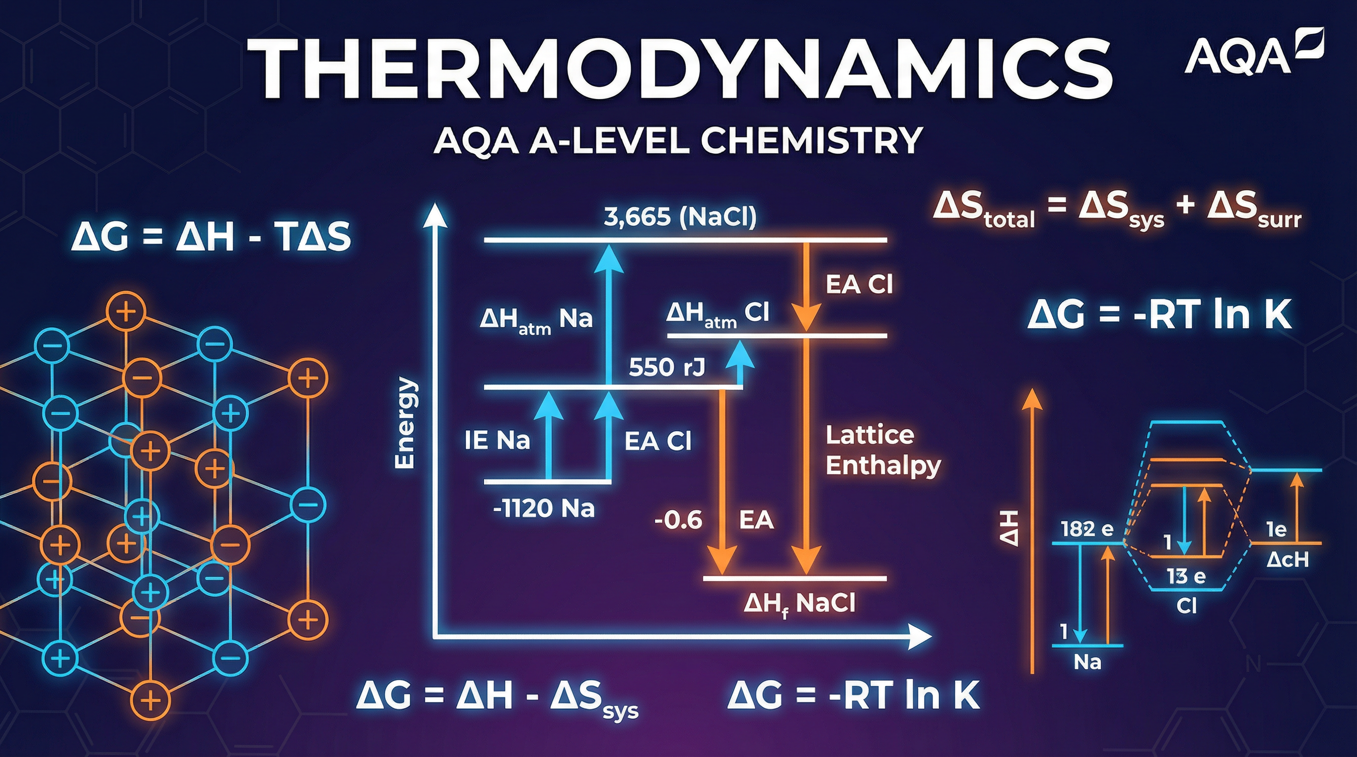
Thermodynamics (AQA 3.1.8) is the powerhouse topic of A-Level Chemistry, combining Born-Haber cycles — which reveal the true strength of ionic bonds through Hess's Law — with Gibbs Free Energy, the ultimate arbiter of whether a reaction can actually occur. Mastering this topic means understanding not just the maths, but the deep physical reasoning behind why ionic compounds form, why some reactions only happen at high temperatures, and why real ionic compounds deviate from the perfect ionic model. Examiners consistently reward candidates who can apply ΔG = ΔH − TΔS with precision and explain covalent character with chemical insight.
## Overview
Thermodynamics sits at the heart of AQA A-Level Chemistry (specification section 3.1.8) and is one of the highest-tariff topics in the entire course. It builds directly on Year 1 enthalpy work and introduces two powerful frameworks: **Born-Haber cycles** for quantifying ionic bond strength through lattice enthalpy, and **Gibbs Free Energy** for determining whether a reaction is thermodynamically feasible. Together, these tools answer two of the most fundamental questions in chemistry — how stable is an ionic compound, and will a given reaction spontaneously occur?
This topic connects to bonding (ionic vs covalent character), electronegativity, periodicity (ionisation energies, atomic radii), and equilibrium (feasibility and spontaneity). In the exam, questions typically appear as multi-part structured questions worth 6–12 marks, combining definition recall (AO1), calculation (AO2), and evaluative explanation (AO3). Candidates who score highest are those who write with precision — including state symbols, correct sign conventions, and explicit unit conversions — and who can explain *why* the theory works, not just apply it mechanically.
---
## Key Concepts
### Concept 1: Lattice Enthalpy and the Born-Haber Cycle
Lattice enthalpy is a measure of the strength of an ionic lattice — the stronger the ionic bonds, the more energy is involved. AQA recognises two related definitions. The **lattice enthalpy of formation** (ΔH°latt) is the enthalpy change when one mole of an ionic solid is formed from its constituent gaseous ions under standard conditions; this is always **exothermic** (negative). The **lattice enthalpy of dissociation** is the reverse process — breaking the lattice into gaseous ions — and is always **endothermic** (positive). Confusing these two is one of the most penalised errors in this topic.
Lattice enthalpy cannot be measured directly in the laboratory, so chemists use an indirect route via a **Born-Haber cycle**, which is simply a specific application of Hess's Law. The cycle connects the lattice enthalpy to a set of measurable enthalpy changes: standard enthalpy of formation, atomisation enthalpies, ionisation energies, and electron affinities.
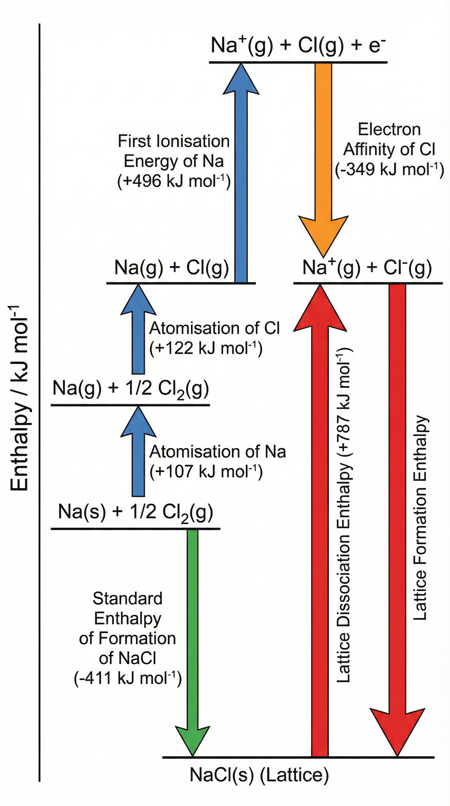
The cycle for NaCl proceeds as follows. Starting from the elements in their standard states (Na(s) and ½Cl₂(g)), we apply: (1) **atomisation of Na** — converting solid sodium to gaseous atoms (+107 kJ mol⁻¹); (2) **atomisation of Cl** — converting ½ mole of Cl₂(g) to Cl(g) (+122 kJ mol⁻¹); (3) **first ionisation energy of Na** — removing one electron from Na(g) to give Na⁺(g) (+496 kJ mol⁻¹); (4) **electron affinity of Cl** — adding one electron to Cl(g) to give Cl⁻(g) (−349 kJ mol⁻¹); and finally (5) **lattice formation enthalpy** — the gaseous ions combine to form the solid lattice (the value we calculate). The **standard enthalpy of formation** of NaCl(s) (−411 kJ mol⁻¹) provides the alternative Hess's Law route. By equating the two routes, the lattice formation enthalpy = −411 − (107 + 122 + 496 − 349) = **−787 kJ mol⁻¹**.
**Key rule for drawing cycles**: endothermic changes are represented by **upward arrows** (energy increases); exothermic changes are represented by **downward arrows** (energy decreases). Arrows must be correctly labelled with the enthalpy change name and value.
---
### Concept 2: Factors Affecting Lattice Enthalpy
Lattice enthalpy magnitude increases with: (a) **increasing ionic charge** — a 2+ or 3+ cation creates much stronger electrostatic attraction than a 1+ cation; and (b) **decreasing ionic radius** — smaller ions can approach each other more closely, increasing the electrostatic force (Coulomb's Law: force ∝ charge₁ × charge₂ / distance²).
This explains why MgO has a much larger lattice enthalpy (−3791 kJ mol⁻¹) than NaCl (−787 kJ mol⁻¹): Mg²⁺ and O²⁻ have double the charge and are smaller than Na⁺ and Cl⁻.
---
### Concept 3: Theoretical vs Experimental Lattice Enthalpy — Covalent Character
The **perfect ionic model** assumes that ions are (i) point charges and (ii) perfectly spherical, with no distortion of electron clouds. Using this model, a theoretical lattice enthalpy can be calculated. However, for many compounds — particularly those with small, highly charged cations or large, polarisable anions — the **experimental lattice enthalpy** (derived from a Born-Haber cycle using real data) differs significantly from the theoretical value.
This discrepancy arises because of **covalent character**. A small, highly charged cation possesses a high **charge density**, which exerts a powerful electric field on adjacent anions. This field **polarises** the anion — distorting its electron cloud towards the cation. The result is partial electron sharing, which is the essence of covalent bonding. The greater the polarisation, the greater the covalent character, and the more the compound's true bonding deviates from the pure ionic model.
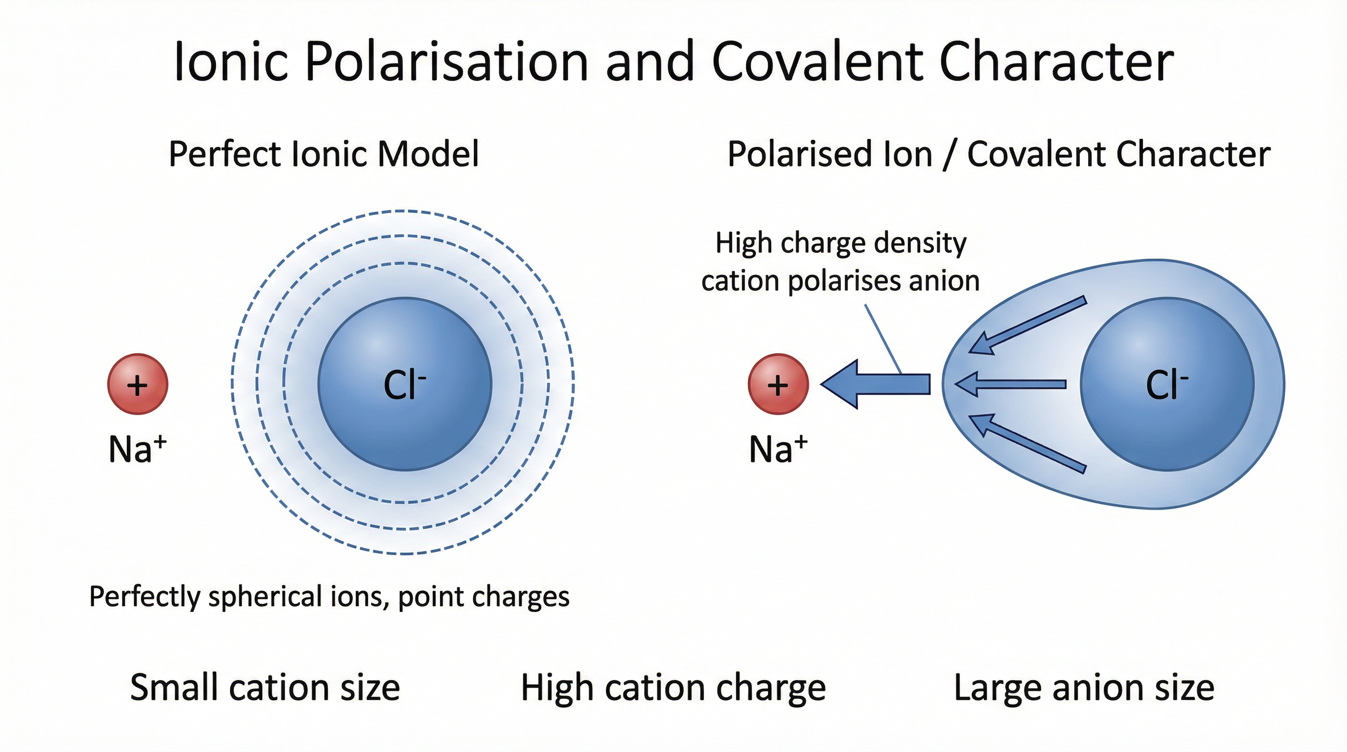
**Fajans' Rules** summarise the factors that increase polarisation and therefore covalent character:
- Small cation (high charge density)
- High cation charge
- Large anion (more polarisable electron cloud)
Aluminium chloride (AlCl₃) is a classic example: Al³⁺ is small and triply charged, giving it very high charge density, which significantly polarises the Cl⁻ ions. The experimental lattice enthalpy is substantially more negative than the theoretical value.
---
### Concept 4: Entropy (ΔS)
Entropy is a measure of the **dispersal of energy** or **disorder** within a system. The greater the number of ways energy can be distributed among particles, the higher the entropy. Key rules for predicting entropy changes:
- **Gases have much higher entropy than liquids or solids** — gas molecules have many more accessible energy states.
- **Dissolving a solid** generally increases entropy (more particles, more disorder).
- **Reactions that increase the number of moles of gas** have positive ΔS.
- **Reactions that decrease the number of moles of gas** have negative ΔS.
The unit of entropy is **J K⁻¹ mol⁻¹** — note joules, not kilojoules. This unit mismatch with enthalpy (kJ mol⁻¹) is the source of the most common calculation error in this topic.
---
### Concept 5: Gibbs Free Energy and Feasibility
The **Gibbs Free Energy equation** is the central equation of this topic:
**ΔG = ΔH − TΔS**
Where ΔG is in kJ mol⁻¹, ΔH is in kJ mol⁻¹, T is in **Kelvin**, and ΔS must be converted to **kJ K⁻¹ mol⁻¹** (divide J K⁻¹ mol⁻¹ values by 1000).
A reaction is **thermodynamically feasible** when **ΔG ≤ 0**. This means the reaction can proceed spontaneously under those conditions. When ΔG > 0, the reaction is not feasible. Note that feasibility does not guarantee that a reaction will actually occur — kinetic barriers (activation energy) may prevent it even when ΔG is negative.
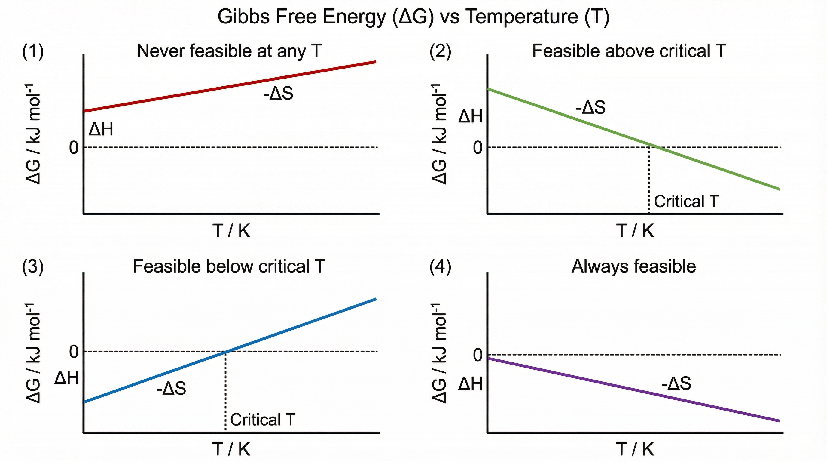
The four scenarios for feasibility depending on the signs of ΔH and ΔS are summarised in the diagram above. The most exam-relevant scenario is when ΔH and ΔS have the same sign, because feasibility then depends on temperature. The **critical temperature** at which ΔG = 0 is found by:
**T_critical = ΔH / ΔS** (using consistent units, both in kJ)
On a graph of ΔG vs T, the relationship is linear with **gradient = −ΔS** and **y-intercept = ΔH**. This graphical interpretation is frequently tested in AQA papers.
---
## Mathematical Relationships
| Formula | Symbols | Status | Notes |
|---|---|---|---|
| **ΔG = ΔH − TΔS** | ΔG (kJ mol⁻¹), ΔH (kJ mol⁻¹), T (K), ΔS (kJ K⁻¹ mol⁻¹) | **Must memorise** | Convert ΔS from J to kJ before substituting |
| **T_crit = ΔH / ΔS** | T (K), ΔH (kJ mol⁻¹), ΔS (kJ K⁻¹ mol⁻¹) | Derived from ΔG = 0 | Both ΔH and ΔS must be in kJ units |
| **ΔH_f = Σ(cycle steps)** | Hess's Law summation | **Must memorise** | Sum of all Born-Haber cycle steps |
| **Gradient of ΔG vs T = −ΔS** | — | Derived | Y-intercept = ΔH |
**Critical unit conversion**: ΔS (J K⁻¹ mol⁻¹) ÷ 1000 = ΔS (kJ K⁻¹ mol⁻¹). Always perform this conversion explicitly in your working.
---
## Practical Applications
Thermodynamics underpins many real-world chemical processes. The **Haber Process** for ammonia synthesis (N₂ + 3H₂ ⇌ 2NH₃) is a classic Gibbs Free Energy problem: ΔH is negative (exothermic) but ΔS is also negative (fewer moles of gas). At low temperatures ΔG is negative and the reaction is feasible, but the rate is too slow; at high temperatures the rate increases but ΔG becomes less negative. The industrial compromise temperature (~450°C) balances feasibility and rate. This synoptic link between thermodynamics and kinetics is a favourite AQA exam theme.
The **Born-Haber cycle** is used industrially to predict the stability of new ionic materials, including battery electrolytes and ceramic superconductors, where lattice enthalpy directly determines thermal stability.