Discrete Random Variables — OCR A-Level Study Guide

 ## Overview Discrete Random Variables (DRVs) are a cornerstone of the OCR A-Level Further Mathematics specification, forming the foundation of statistical distributions. A DRV is a variable that can only take on a countable number of distinct values, each with an associated probability. Think of the score from a single roll of a die or the number of heads in three coin tosses. This topic is not just about calculation; it's about deep conceptual understanding, particularly concerning the algebra of expectation and variance. Examiners frequently test the subtle but critical differences between scaling a single variable (like 2X) and summing independent variables (like X₁ + X₂). Mastery here is essential as these principles are built upon in later topics like the Binomial, Geometric, and Poisson distributions. Expect to see questions ranging from finding a constant in a probability distribution to complex, multi-part problems involving linear combinations of variables.  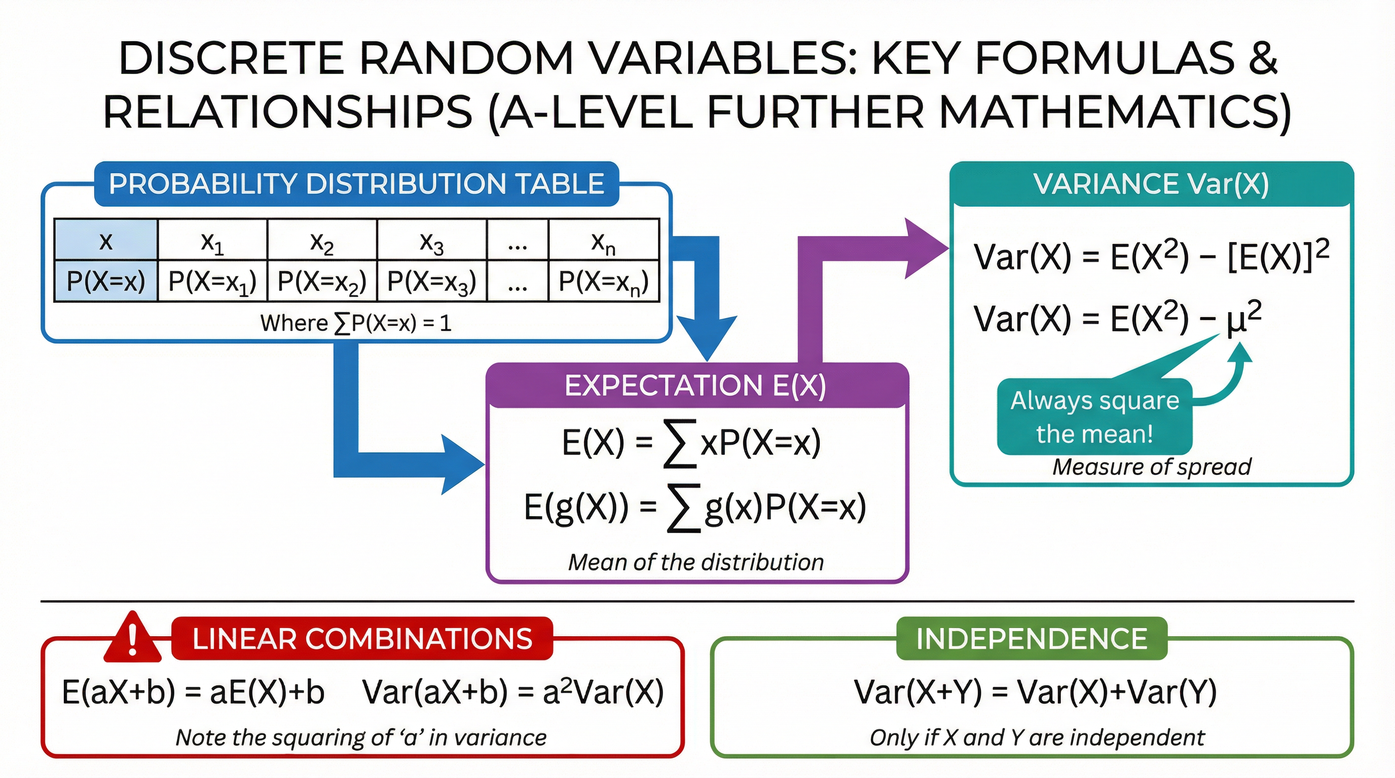## Key Concepts ### Concept 1: Probability Distributions A probability distribution for a discrete random variable X is a table or function that maps each possible value of X to its probability. For a distribution to be valid, two conditions must be met: 1. **0 ≤ P(X=x) ≤ 1** for all values of x. (Each probability must be between 0 and 1). 2. **ΣP(X=x) = 1**. (The sum of all probabilities must equal 1). Examiners often test the second condition by giving you a probability distribution with an unknown constant (e.g., 'k') and asking you to find its value. Your first step should always be to sum the probabilities and set them equal to 1. **Example**: A DRV, X, has the probability distribution shown below. | x | 1 | 2 | 3 | 4 | |------|-----|-----|-----|------| | P(X=x)| 0.1 | k | 0.3 | 0.4 | To find k, we use ΣP(X=x) = 1: 0.1 + k + 0.3 + 0.4 = 1 k + 0.8 = 1 k = 0.2 ### Concept 2: Expectation (Mean) The expectation of a DRV, denoted E(X), is its theoretical long-run average. It's a weighted mean of the possible values, where the weights are the probabilities. **Formula**: E(X) = ΣxP(X=x) This means you multiply each value (x) by its corresponding probability (P(X=x)) and sum the results. The expectation doesn't have to be one of the possible values of X. We can also find the expectation of a function of X, g(X). **Formula**: E(g(X)) = Σg(x)P(X=x) A particularly important case is E(X²), which is crucial for calculating variance. **Example**: Using the distribution above with k=0.2: E(X) = (1 × 0.1) + (2 × 0.2) + (3 × 0.3) + (4 × 0.4) = 0.1 + 0.4 + 0.9 + 1.6 = 3.0 E(X²) = (1² × 0.1) + (2² × 0.2) + (3² × 0.3) + (4² × 0.4) = 0.1 + 0.8 + 2.7 + 6.4 = 10.0 ### Concept 3: Variance and Standard Deviation Variance, denoted Var(X), measures the spread or dispersion of the distribution around the mean. A small variance means the data points are clustered close to the mean, while a large variance indicates they are spread out. **Formula**: Var(X) = E(X²) - [E(X)]² This is often remembered as **"the mean of the squares minus the square of the mean"**. This is a critical formula to memorise and apply correctly. A common mistake is to calculate E(X²) and forget to subtract the square of E(X). **Standard Deviation (σ)** is simply the square root of the variance. It is useful because it is in the same units as the original data. **Formula**: σ = √Var(X) **Example**: Using our ongoing example: Var(X) = E(X²) - [E(X)]² = 10.0 - (3.0)² = 10.0 - 9.0 = 1.0 Standard Deviation = √1.0 = 1.0  ### Concept 4: Linear Combinations of a Random Variable This is where the Further Maths content really begins. What happens to the mean and variance if we transform the variable X into a new variable Y = aX + b, where 'a' and 'b' are constants? **Expectation**: E(aX + b) = aE(X) + b *The expectation is affected by both the scaling factor 'a' and the shifting constant 'b'.* **Variance**: Var(aX + b) = a²Var(X) *The variance is only affected by the scaling factor 'a', and crucially, this factor is **squared**. The shifting constant 'b' has no effect on the spread of the data.* This is a major source of errors. Candidates often forget to square the 'a'. ### Concept 5: Sums of Independent Random Variables If we have two **independent** random variables, X and Y, we can find the expectation and variance of their sum. **Expectation**: E(X + Y) = E(X) + E(Y) **Variance**: Var(X + Y) = Var(X) + Var(Y) *(This only holds if X and Y are independent)* Examiners will award a specific mark (B1) for stating the independence assumption when using this formula. 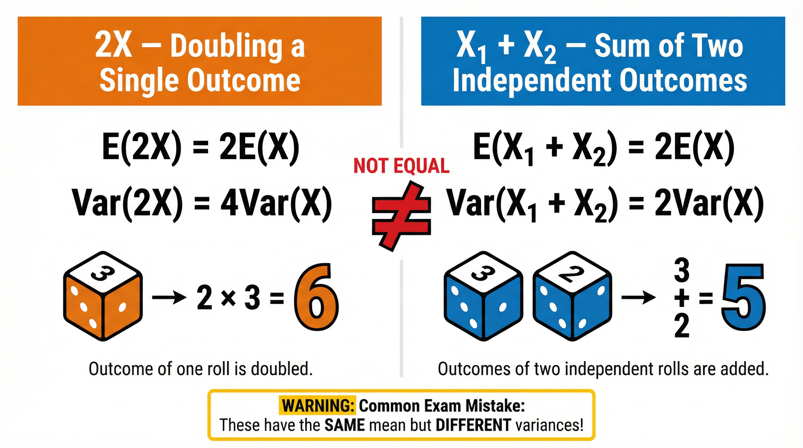### The 2X vs X₁ + X₂ Trap This is a classic exam question designed to test your understanding of the concepts above. Let X₁ and X₂ be two independent observations of the same random variable X. | | **2X (Doubling a single outcome)** | **X₁ + X₂ (Sum of two independent outcomes)** | |--------------|------------------------------------|------------------------------------------------| | **Expectation**| E(2X) = 2E(X) | E(X₁ + X₂) = E(X₁) + E(X₂) = 2E(X) | | **Variance** | Var(2X) = 2²Var(X) = **4Var(X)** | Var(X₁ + X₂) = Var(X₁) + Var(X₂) = **2Var(X)** | **The key takeaway**: The means are the same, but the variances are different. This is a high-level distinction that separates top candidates.  ## Mathematical/Scientific Relationships - **Validity Check**: ΣP(X=x) = 1 *(Must memorise)* - **Expectation**: E(X) = ΣxP(X=x) *(Given on formula sheet)* - **Expectation of a function**: E(g(X)) = Σg(x)P(X=x) *(Given on formula sheet)* - **Variance**: Var(X) = E(X²) - [E(X)]² *(Given on formula sheet)* - **Linear Combination (Expectation)**: E(aX + b) = aE(X) + b *(Must memorise)* - **Linear Combination (Variance)**: Var(aX + b) = a²Var(X) *(Must memorise)* - **Sum of Independent Variables (Expectation)**: E(X + Y) = E(X) + E(Y) *(Must memorise)* - **Sum of Independent Variables (Variance)**: Var(X + Y) = Var(X) + Var(Y) *(Must memorise, requires independence)* ## Practical Applications Discrete random variables are the backbone of risk analysis and modelling in many fields: - **Insurance**: An insurance company might model the number of claims it receives in a month as a DRV to calculate expected payouts and set premiums. - **Quality Control**: A factory could use a DRV to model the number of defective items in a batch, helping to monitor and control production quality. - **Finance**: In financial modelling, the number of times a stock price moves up or down in a day can be treated as a DRV to assess volatility and risk. - **Genetics**: The number of offspring with a particular genetic trait can be modelled as a DRV.