Probability Generating Functions Revision Notes
Subject: Further Mathematics | Level: A-Level | Exam Board: OCR
Master one of the most powerful tools in A-Level Further Maths. This guide breaks down Probability Generating Functions (PGFs), showing you how to encode entire distributions into a single function, then differentiate to find the mean and variance. It’s your key to unlocking top marks in OCR exam questions on discrete distributions.
Revision Notes & Key Concepts
Key Terms & Definitions
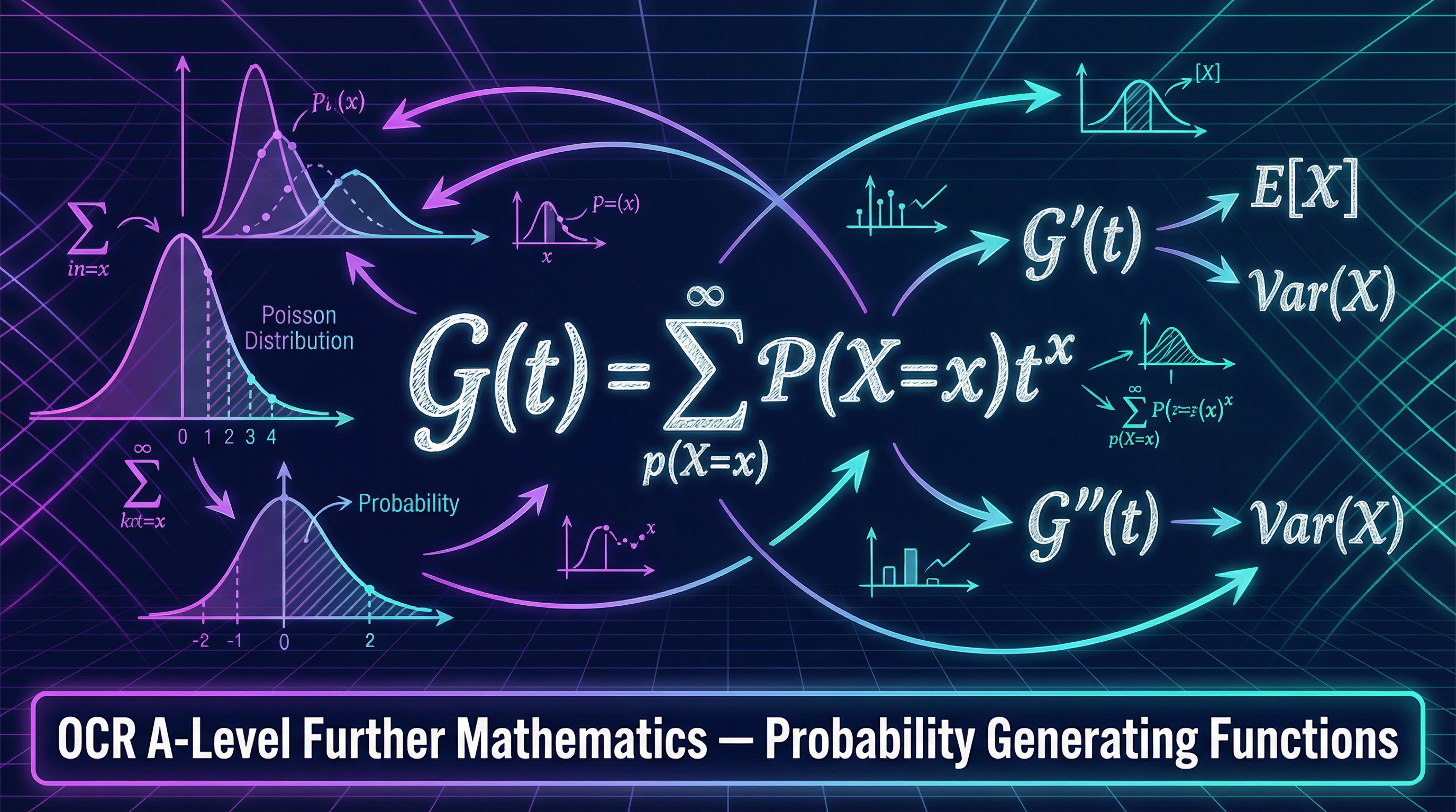
- Probability Generating Function (PGF)
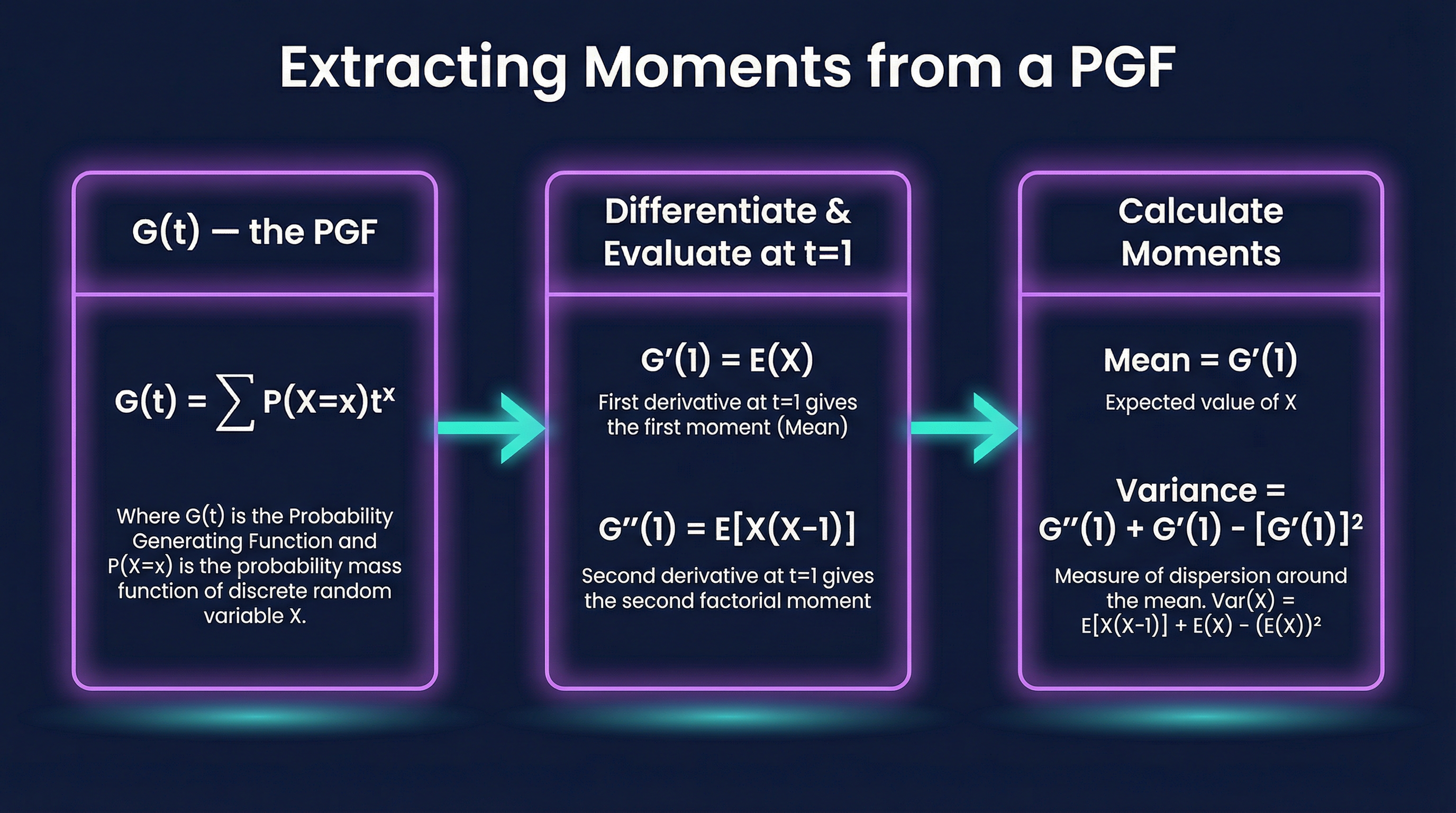
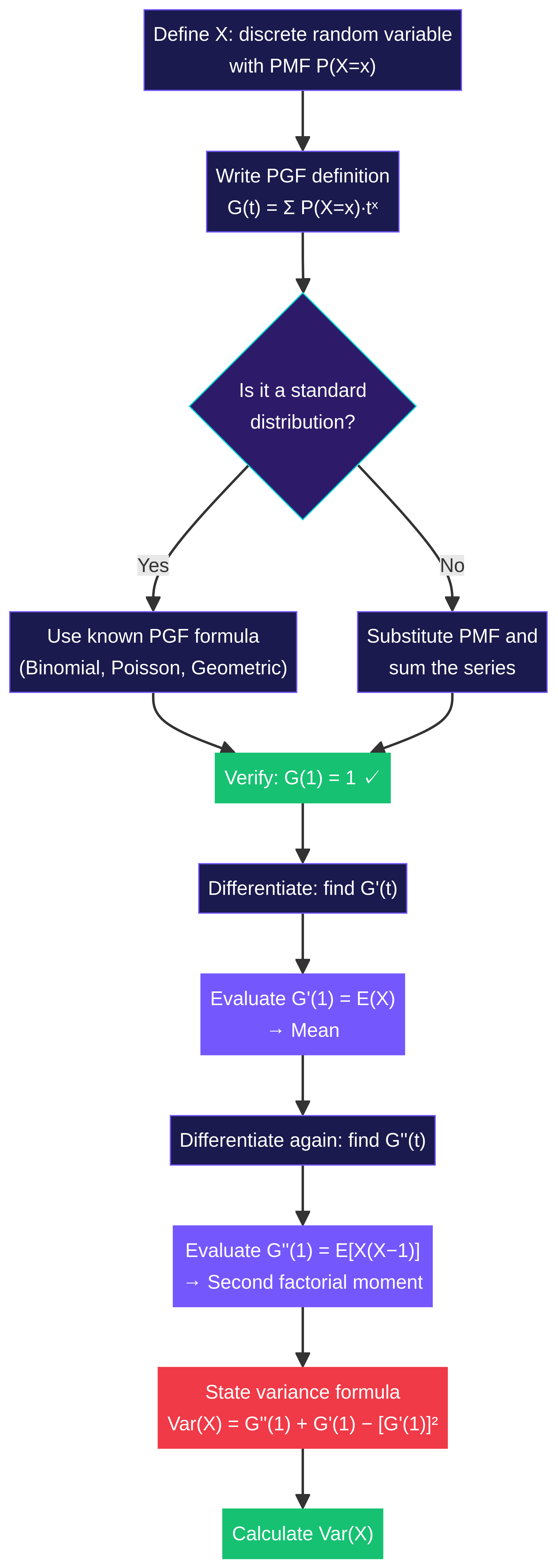
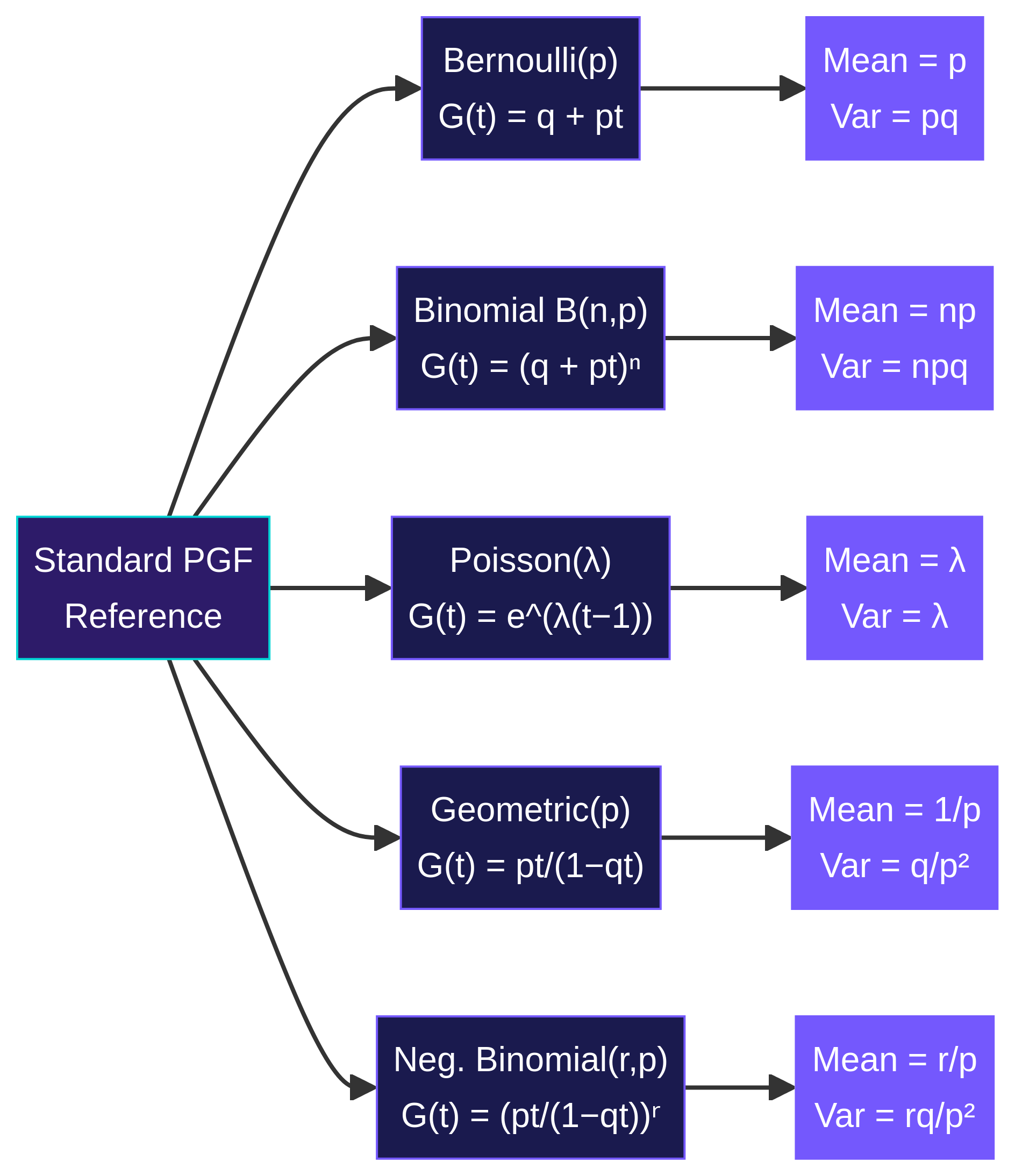
- For a discrete random variable X, the PGF is G(t) = E(tˣ) = Σ P(X=x)tˣ, where the sum is over all values x that X can take.
- Moment
- A quantitative measure of the shape of a probability distribution. The first moment is the mean. The second central moment is the variance.
- Factorial Moment
- The r-th factorial moment of X is E[X(X-1)...(X-r+1)]. The second factorial moment, E[X(X-1)], is found from G''(1).
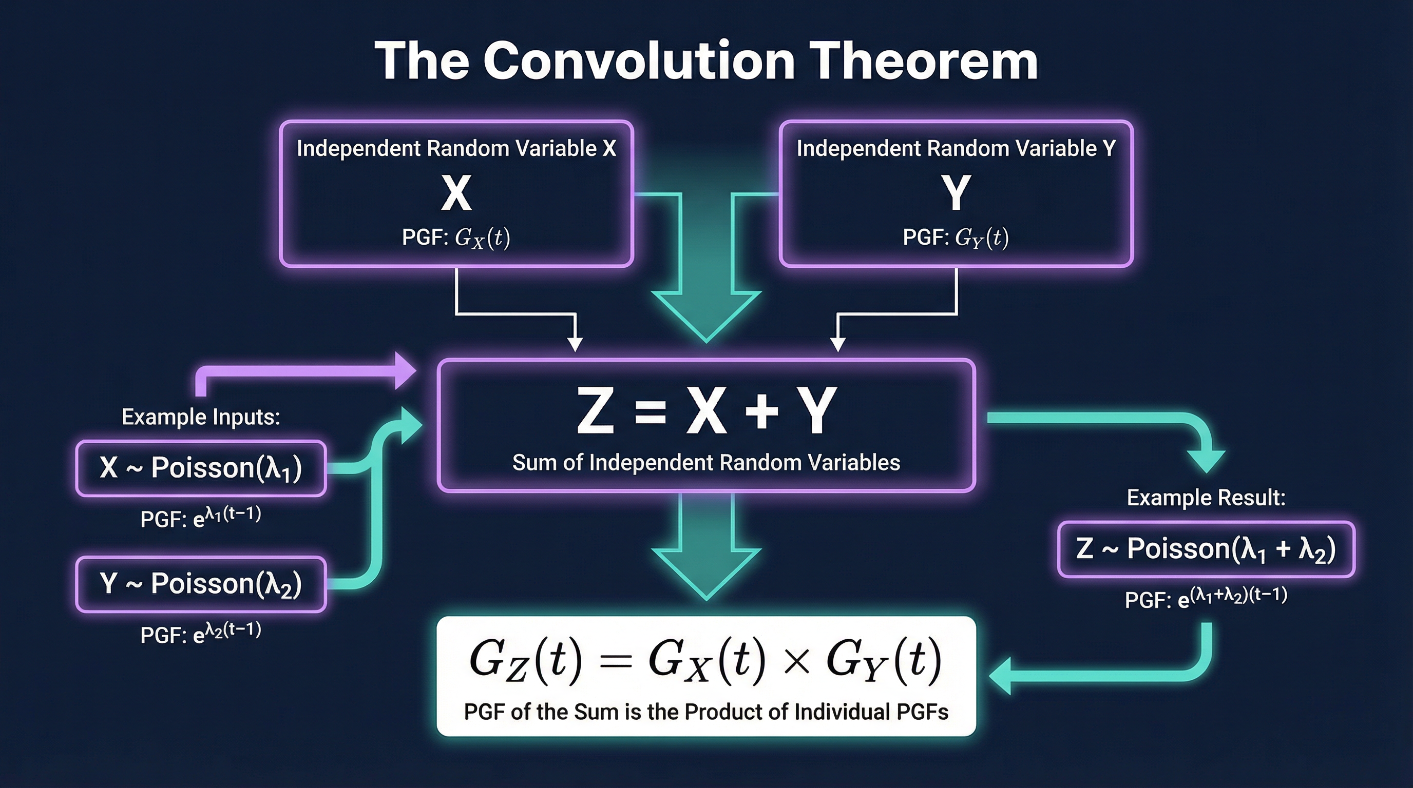
- Convolution Theorem
- If X and Y are independent random variables, the PGF of their sum Z = X + Y is the product of their individual PGFs: G_Z(t) = G_X(t) * G_Y(t).
- PMF (Probability Mass Function)
- A function that gives the probability that a discrete random variable is exactly equal to some value. P(X=x).
- Dummy Variable
- A variable, such as 't' in G(t), that is used as a placeholder in a function and is not one of the variables being measured.
Worked Examples
Worked Example
Question: The discrete random variable X has a Poisson distribution with mean 2. The discrete random variable Y has a Poisson distribution with mean 3. X and Y are independent. Find the probability generating function of Z = X + Y and use it to find P(Z=4).
Solution: Step 1: Write down the PGFs for X and Y. For X ~ Po(2), G_X(t) = e^(2(t-1)). For Y ~ Po(3), G_Y(t) = e^(3(t-1)). Step 2: Use the convolution theorem for the sum of independent variables. Since Z = X + Y and X, Y are independent, G_Z(t) = G_X(t) * G_Y(t). G_Z(t) = e^(2(t-1)) * e^(3(t-1)) = e^(2(t-1) + 3(t-1)) = e^(5(t-1)). Step 3: Identify the distribution of Z. The PGF G_Z(t) = e^(5(t-1)) is the standard PGF for a Poisson distribution with parameter 5. Therefore, Z ~ Po(5). Step 4: Calculate P(Z=4) using the identified distribution. For Z ~ Po(5), the PMF is P(Z=z) = e⁻⁵ * 5ᶻ / z! P(Z=4) = e⁻⁵ * 5⁴ / 4! = (625 * e⁻⁵) / 24. Step 5: Calculate the final numerical answer. P(Z=4) ≈ 0.175467... Final answer: **0.175** (to 3 s.f.)
Worked Example
Question: A discrete random variable X has probability generating function G_X(t) = k(1 + 2t + 3t²). (i) Find the value of the constant k. (ii) Use the PGF to find the mean and variance of X.
Solution: (i) Step 1: Use the property that G(1) = 1. G_X(1) = k(1 + 2(1) + 3(1)²) = k(1 + 2 + 3) = 6k. Since G_X(1) must equal 1, we have 6k = 1, so **k = 1/6**. (ii) Step 2: Find the first derivative, G'(t). G_X(t) = (1/6)(1 + 2t + 3t²) G'_X(t) = (1/6)(2 + 6t). Step 3: Calculate the mean, E(X) = G'(1). E(X) = G'_X(1) = (1/6)(2 + 6(1)) = 8/6 = **4/3**. Step 4: Find the second derivative, G''(t). G''_X(t) = (1/6)(6) = 1. Step 5: Calculate G''(1). G''_X(1) = 1. This is the value of E[X(X-1)]. Step 6: State and use the variance formula. Var(X) = G''(1) + G'(1) - [G'(1)]² Var(X) = 1 + (4/3) - (4/3)² Var(X) = 1 + 4/3 - 16/9 = 9/9 + 12/9 - 16/9 = **5/9**.
Worked Example
Question: The number of emails arriving at an office follows a Poisson distribution with a mean of 3 per hour. Use probability generating functions to find the probability that exactly 5 emails arrive in a two-hour period.
Solution: Step 1: Define the random variables for each hour. Let X₁ be the number of emails in the first hour, X₁ ~ Po(3). Let X₂ be the number of emails in the second hour, X₂ ~ Po(3). We assume the number of arrivals in each hour is independent. Step 2: Write down the PGF for a single hour. For X₁ and X₂, the PGF is G(t) = e^(3(t-1)). Step 3: Find the PGF for the total number of emails in two hours. Let Z = X₁ + X₂. By the convolution theorem, G_Z(t) = G_X₁(t) * G_X₂(t). G_Z(t) = e^(3(t-1)) * e^(3(t-1)) = e^(6(t-1)). Step 4: Identify the distribution of Z and calculate the probability. The PGF G_Z(t) shows that Z ~ Po(6). P(Z=5) = e⁻⁶ * 6⁵ / 5! = (7776 * e⁻⁶) / 120 = **0.161** (to 3 s.f.).
Practice Questions
Question: A fair four-sided die is numbered 1, 2, 3, 4. The result of a single roll is the random variable X. Find the probability generating function of X.
Answer:
Question: A random variable X has PGF G(t) = (0.4 + 0.6t)¹⁰. Identify the distribution of X, stating its parameters, and find E(X).
Answer:
Question: The random variable Y has PGF G(t) = e^(4(t-1)). Use differentiation to find the variance of Y.
Answer:
Question: Let X be a random variable with PGF G_X(t). A second random variable is defined as Y = 2X + 3. Find the PGF of Y, G_Y(t), in terms of G_X(t).
Answer:
Question: A discrete random variable X has PGF G(t) = (1/35)(1 + 4t + 10t² + 20t³). Find the mode of X.
Answer: