Subject: Mathematics | Level: GCSE | Exam Board: AQA
Master probability for your GCSE Mathematics exam. This comprehensive guide covers everything from basic chance and the probability scale to complex tree diagrams, Venn diagrams, and conditional probability, ensuring you secure those vital marks.
Revision Notes & Key Concepts
Revision Podcast Transcript
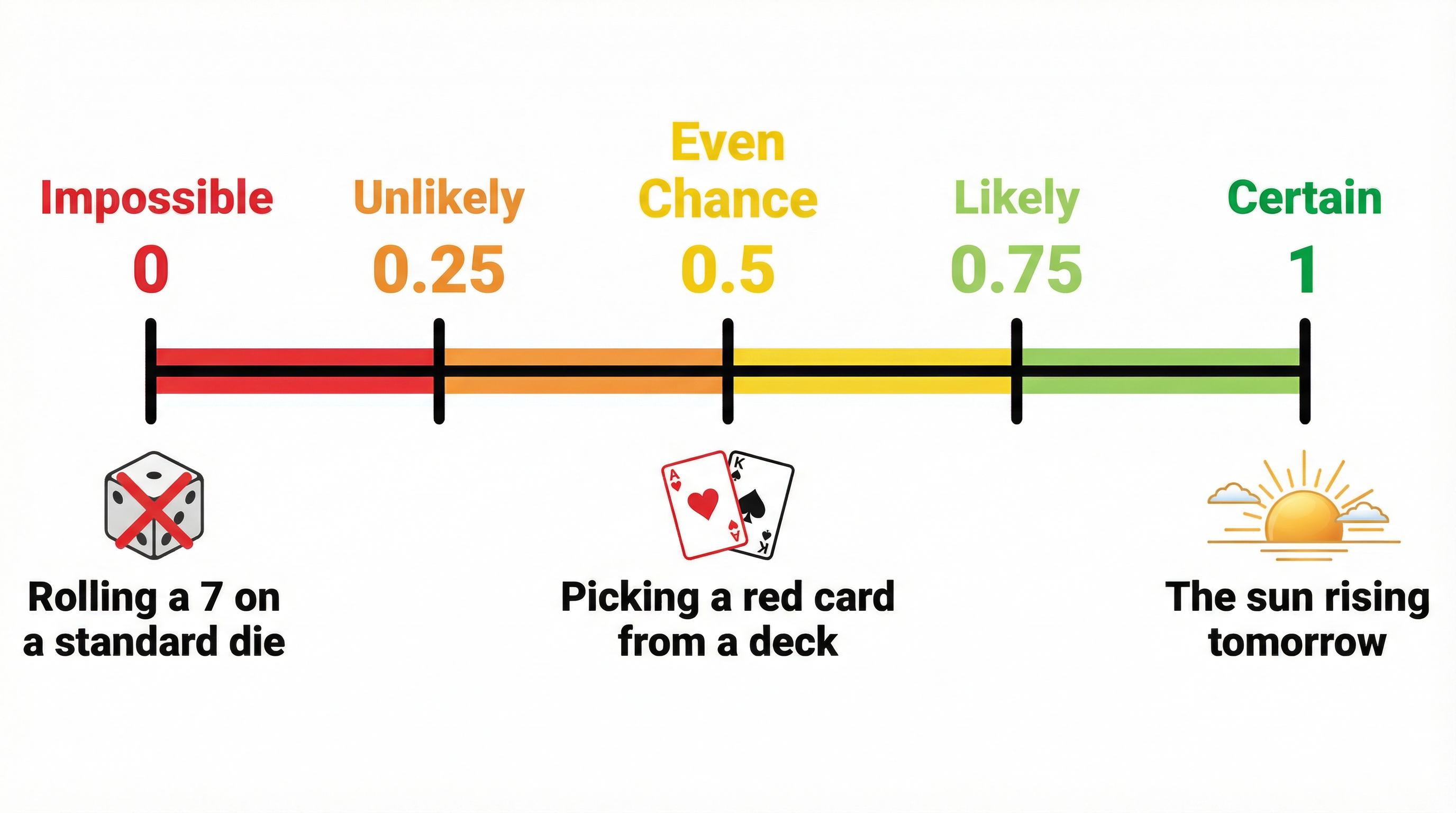
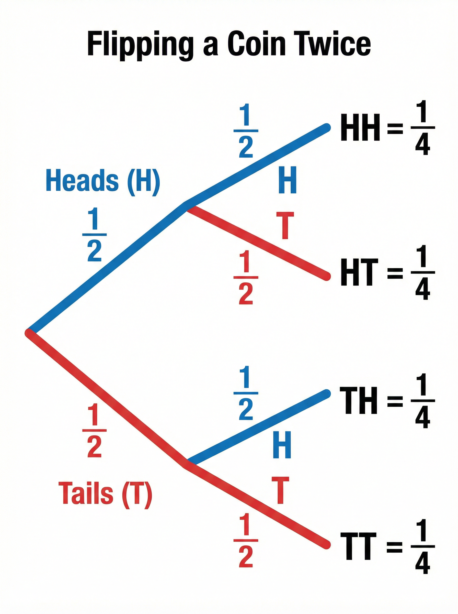
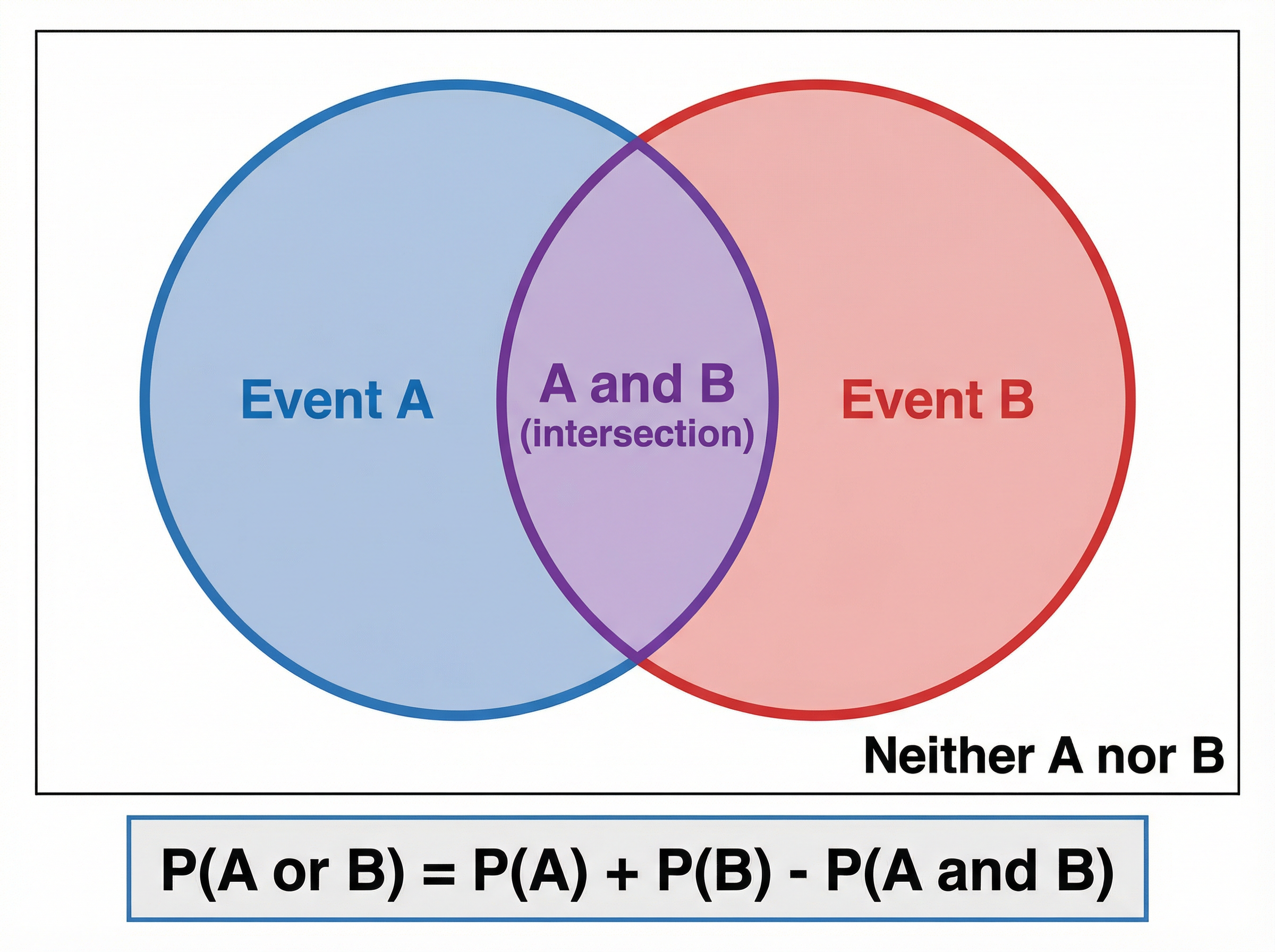
Welcome to your GCSE Maths revision podcast. I'm your tutor, and today we're diving into one of the most consistently examined topics across all GCSE Maths papers: Probability. Whether you're sitting AQA, Edexcel, OCR, or any other board, probability questions appear on almost every paper, and the good news is that with the right approach, they are absolutely achievable marks. So settle in, grab a pen, and let's get started. Let's begin with the big picture. What is probability? At its heart, probability is the mathematics of chance. It gives us a way to measure how likely an event is to happen, using a scale from zero to one. Zero means something is impossible — it simply cannot happen. One means something is certain — it will definitely happen. Everything else sits somewhere in between. You might also see probabilities written as fractions, decimals, or percentages, and you need to be comfortable converting between all three. Now, the fundamental formula you absolutely must know is this: the probability of an event equals the number of favourable outcomes divided by the total number of possible outcomes. Write that down. P of A equals favourable outcomes over total outcomes. This is your starting point for almost every probability question at GCSE. Let's make that concrete. Imagine a bag containing three red balls and five blue balls. What is the probability of picking a red ball at random? The number of favourable outcomes — that's the red balls — is three. The total number of outcomes is eight, because there are eight balls altogether. So the probability is three over eight. Simple as that. Now let's move on to one of the most important concepts: complementary events. The probability that something does NOT happen is one minus the probability that it does happen. So if the probability of picking a red ball is three eighths, then the probability of NOT picking a red ball is one minus three eighths, which equals five eighths. Examiners love testing this, often by giving you the probability of one event and asking for the probability of the other. Always check: do your probabilities add up to one? If they don't, you've made an error somewhere. Next up: mutually exclusive events. Two events are mutually exclusive if they cannot both happen at the same time. For example, when you roll a single die, you cannot roll a three AND a five on the same roll. They're mutually exclusive. For mutually exclusive events, the addition rule applies: the probability of A or B happening equals the probability of A plus the probability of B. This is sometimes called the OR rule. Remember: OR means ADD — but only when the events are mutually exclusive. Now, what about independent events? Two events are independent if the outcome of one does not affect the outcome of the other. Flipping a coin and rolling a die are independent — the coin doesn't care what the die does. For independent events, we use the multiplication rule: the probability of A AND B both happening equals the probability of A multiplied by the probability of B. AND means MULTIPLY. This is one of the most important rules in probability, and it comes up constantly in exam questions. Here's a worked example. A fair coin is flipped and a fair six-sided die is rolled. What is the probability of getting heads AND rolling a six? The probability of heads is one half. The probability of rolling a six is one sixth. Because these are independent events, we multiply: one half times one sixth equals one twelfth. That's your answer. Now let's talk about tree diagrams, which are a fantastic tool for organising probability problems involving two or more events. A tree diagram shows all possible outcomes of a sequence of events, with probabilities written on each branch. The key rules are: probabilities along each branch must add up to one, and to find the probability of a combined outcome, you multiply along the branches. To find the probability of multiple outcomes, you add the relevant end probabilities together. Let me walk you through a tree diagram example. A bag contains four red and two blue counters. A counter is picked at random, its colour noted, and then it is replaced. A second counter is then picked. What is the probability that both counters are the same colour? First, let's set up the tree. On the first pick: probability of red is four sixths, which simplifies to two thirds. Probability of blue is two sixths, which simplifies to one third. Because the counter is replaced, the probabilities on the second pick are the same. So from the red branch: probability of red again is two thirds, probability of blue is one third. From the blue branch: probability of red is two thirds, probability of blue is one third. Now, both counters the same colour means either red then red, or blue then blue. Red then red: two thirds times two thirds equals four ninths. Blue then blue: one third times one third equals one ninth. Add these together: four ninths plus one ninth equals five ninths. That's the answer. Now, what if the counter is NOT replaced? This is called sampling without replacement, and it changes the probabilities on the second pick because there are now fewer counters in the bag. This is a Higher tier concept and it's where many candidates lose marks — they forget to adjust the denominator. Always ask yourself: is this with replacement or without replacement? Let's move on to Venn diagrams, another key tool for probability. A Venn diagram uses overlapping circles inside a rectangle to show sets of outcomes. The rectangle represents the entire sample space — all possible outcomes. Each circle represents an event. The overlapping region shows outcomes that belong to both events simultaneously. Key notation to know: P of A union B — that's A or B — equals the probability of being in either circle or both. P of A intersection B — that's A and B — equals the probability of being in the overlapping region only. P of A prime — that's not A — equals everything outside circle A. The addition formula for Venn diagrams is: P of A or B equals P of A plus P of B minus P of A and B. We subtract the intersection because otherwise we'd count it twice. Let's also cover frequency trees and relative frequency, which appear on Foundation papers. Relative frequency is an experimental estimate of probability based on repeated trials. The formula is: relative frequency equals frequency of the event divided by total number of trials. The more trials you conduct, the closer your relative frequency gets to the true theoretical probability. Examiners often ask you to comment on this — a good answer will say something like: as the number of trials increases, the relative frequency converges towards the theoretical probability. Right, now let's talk exam technique, because knowing the maths is only half the battle. First: always show your working. In probability questions, method marks are available even if your final answer is wrong. If you set up a tree diagram correctly but make an arithmetic error, you can still earn marks. Never just write down an answer without showing how you got there. Second: check that your probabilities are valid. A probability can never be less than zero or greater than one. If you get an answer of 1.3 or negative 0.2, you've definitely made an error. Go back and check. Third: watch out for the replacement trap. This is one of the most common errors in GCSE probability. When a question says "without replacement", the denominator changes on the second pick. Candidates who forget this will lose marks. Underline the words "with replacement" or "without replacement" as soon as you read the question. Fourth: read the question carefully for the word "given". Conditional probability — where you're told one event has already happened — is a Higher tier topic. The notation P of B given A means: what is the probability of B, given that A has already occurred? In a Venn diagram, this means you restrict your sample space to just the circle for A, then find the proportion that also satisfies B. Fifth: when using tree diagrams, always label your branches clearly with both the outcome and the probability. Examiners award marks for correct probabilities on branches, so even if your final answer is wrong, you can still pick up marks for a correctly structured diagram. Sixth: don't forget to simplify fractions unless the question asks for a decimal or percentage. Leaving an answer as twelve over forty-eight when it should be one quarter is sloppy and could cost you a mark. Now let's do a quick-fire recall quiz. Pause after each question and try to answer before I give you the answer. Question one: What is the probability scale, and what do zero and one represent? The scale runs from zero to one. Zero means impossible. One means certain. Question two: What is the formula for basic probability? P of A equals number of favourable outcomes divided by total number of outcomes. Question three: If P of A equals 0.3, what is P of not A? One minus 0.3 equals 0.7. Question four: What rule do you use for independent events where both must happen? The multiplication rule: P of A and B equals P of A times P of B. Question five: In a tree diagram, how do you find the probability of a combined outcome? Multiply along the branches. Question six: What is relative frequency? Frequency of an event divided by total number of trials — an experimental estimate of probability. Question seven: What changes when sampling without replacement? The denominator decreases on subsequent picks because there are fewer items in the bag. Question eight: State the addition rule for mutually exclusive events. P of A or B equals P of A plus P of B. How did you do? If you struggled with any of those, go back to that section and re-read it before your exam. Let's wrap up with a quick summary of the key things to remember. One: probability is always between zero and one inclusive. Two: P of not A equals one minus P of A. Three: for mutually exclusive events, OR means ADD. Four: for independent events, AND means MULTIPLY. Five: in tree diagrams, multiply along branches and add between branches. Six: always check whether sampling is with or without replacement. Seven: relative frequency is an estimate that improves with more trials. Eight: show all working — method marks are there to be earned. That's it for today's podcast on Probability. You've covered the probability scale, basic probability, complementary events, mutually exclusive and independent events, tree diagrams, Venn diagrams, and relative frequency. These topics come up on virtually every GCSE Maths paper, so the time you've invested today will pay off in the exam. Keep practising past paper questions, check your answers against the mark scheme, and remember — every mark counts. Good luck, and I'll see you in the next episode.
Key Terms & Definitions
- Mutually Exclusive
- Events that cannot happen at the same time.
- Independent Events
- Events where the outcome of one does not affect the outcome of the other.
- Relative Frequency
- An estimate of probability based on experimental data (successful trials ÷ total trials).
- Sample Space
- The set of all possible outcomes of an experiment.
- Complementary Event
- The event that something does not happen. P(A') = 1 - P(A).
- Biased
- Not fair; the outcomes are not equally likely.
Worked Examples
Worked Example
Question: A bag contains 5 red counters, 3 blue counters and 2 green counters. A counter is taken at random from the bag. State the probability that the counter is blue. (1 mark)
Solution: Step 1: Calculate the total number of counters. Total = 5 + 3 + 2 = 10. Step 2: Identify the number of blue counters. Number of blue = 3. Step 3: Write as a fraction. Final answer: 3/10
Worked Example
Question: The probability that a biased coin lands on heads is 0.65. The coin is flipped 200 times. Calculate an estimate for the number of times the coin will land on heads. (2 marks)
Solution: Step 1: Use the expected frequency formula: Expected frequency = Probability × Number of trials. Step 2: Substitute the values. Expected frequency = 0.65 × 200 Step 3: Calculate the result. 0.65 × 100 = 65, so 0.65 × 200 = 130. Final answer: 130
Worked Example
Question: There are 4 red pens and 6 blue pens in a pencil case. Two pens are taken at random without replacement. Calculate the probability that both pens are the same colour. (4 marks)
Solution: Step 1: Identify the total number of pens initially. Total = 10. Step 2: Calculate the probability of picking Red then Red (RR). P(1st is Red) = 4/10 Since it's without replacement, there are now 3 red pens left out of 9 total. P(2nd is Red) = 3/9 P(RR) = (4/10) × (3/9) = 12/90 Step 3: Calculate the probability of picking Blue then Blue (BB). P(1st is Blue) = 6/10 Without replacement, there are now 5 blue pens left out of 9 total. P(2nd is Blue) = 5/9 P(BB) = (6/10) × (5/9) = 30/90 Step 4: Add the probabilities of the mutually exclusive successful outcomes. P(Same colour) = P(RR) + P(BB) = 12/90 + 30/90 = 42/90 Step 5: Simplify the fraction. 42/90 = 7/15 Final answer: 7/15
Practice Questions
Question: A spinner has sections coloured red, blue, green, and yellow. The probability of landing on red is 0.3. The probability of landing on blue is 0.2. The probability of landing on green is 0.15. Calculate the probability of landing on yellow. (2 marks)
Answer:
Question: In a class of 30 students, 18 study French, 15 study Spanish, and 5 study neither. A student is chosen at random. Find the probability that the student studies both French and Spanish. (3 marks)
Answer:
Question: A box contains 7 chocolate biscuits and 3 toffee biscuits. Sarah takes a biscuit at random and eats it. She then takes a second biscuit at random and eats it. Calculate the probability that she eats one of each type of biscuit. (4 marks)
Answer:
Question: A factory produces lightbulbs. A sample of 500 lightbulbs is tested, and 12 are found to be defective. The factory produces 25,000 lightbulbs in a week. Estimate the total number of defective lightbulbs produced in that week. (3 marks)
Answer:
Question: Events A and B are independent. P(A) = 0.4 and P(A and B) = 0.12. Work out P(B). (2 marks)
Answer: