Subject: Mathematics | Level: GCSE | Exam Board: AQA
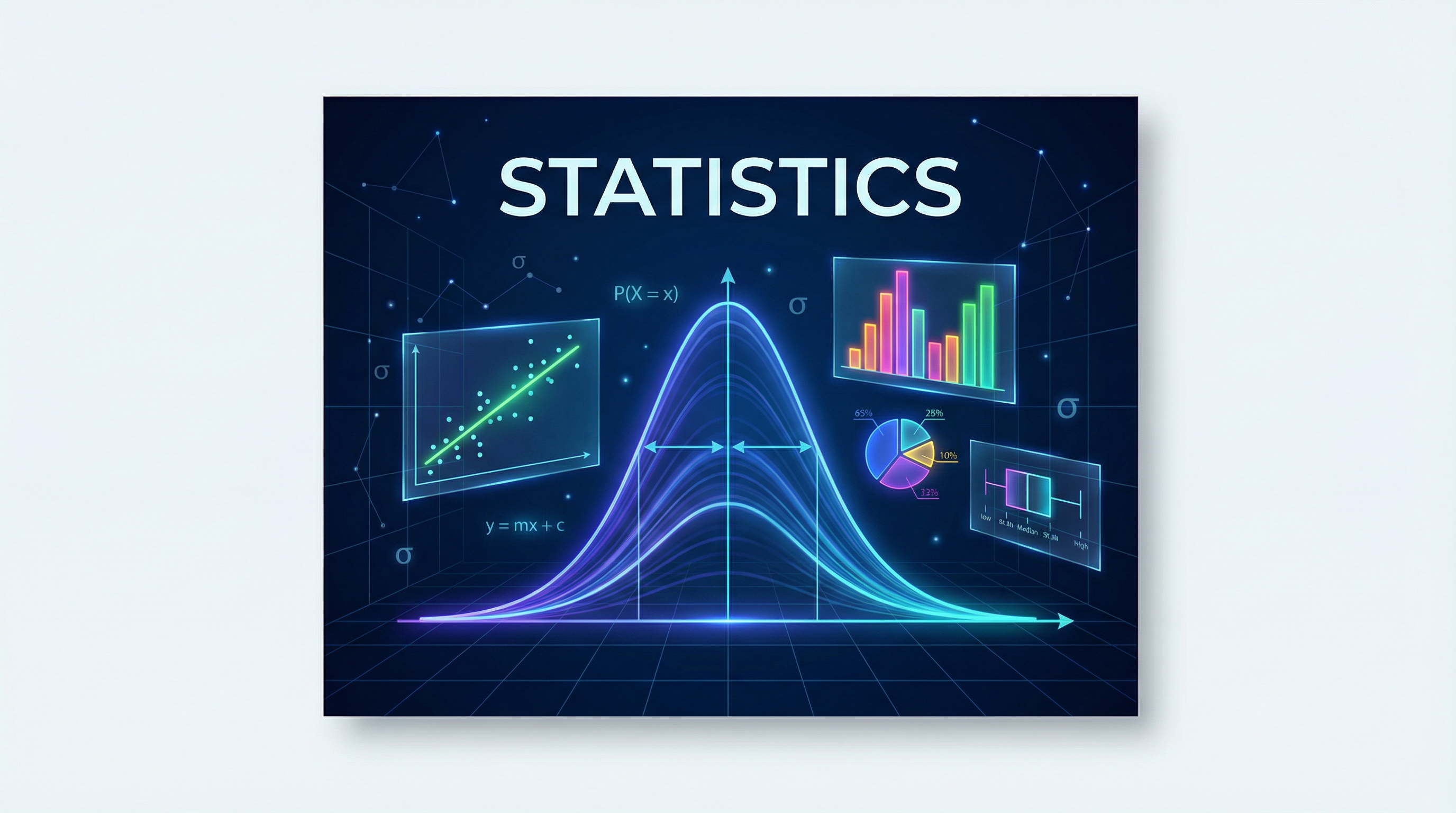
Statistics is the science of collecting, analysing, and interpreting data. It is a highly practical and mark-friendly topic that appears in every single GCSE and A-Level Mathematics paper.
Revision Notes & Key Concepts
Key Terms & Definitions
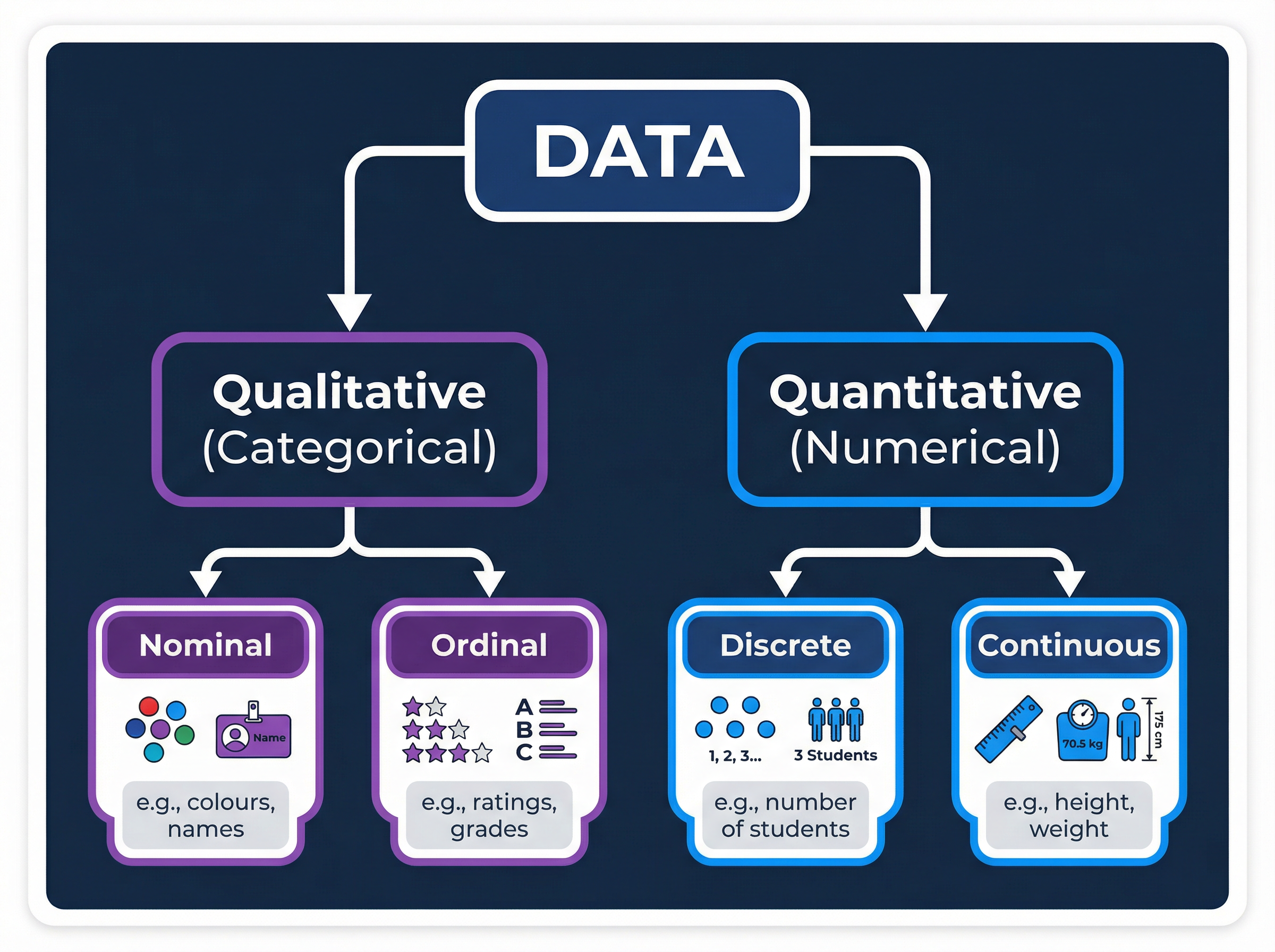
- Continuous Data
- Data that can take any numerical value within a given range, typically obtained by measuring.
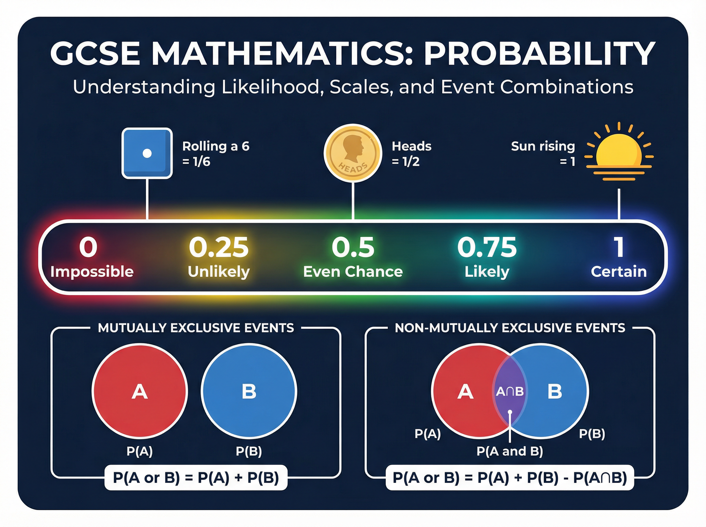
- Mutually Exclusive Events
- Events that cannot occur at the same time.
- Independent Events
- Events where the outcome of one does not affect the probability of the other.
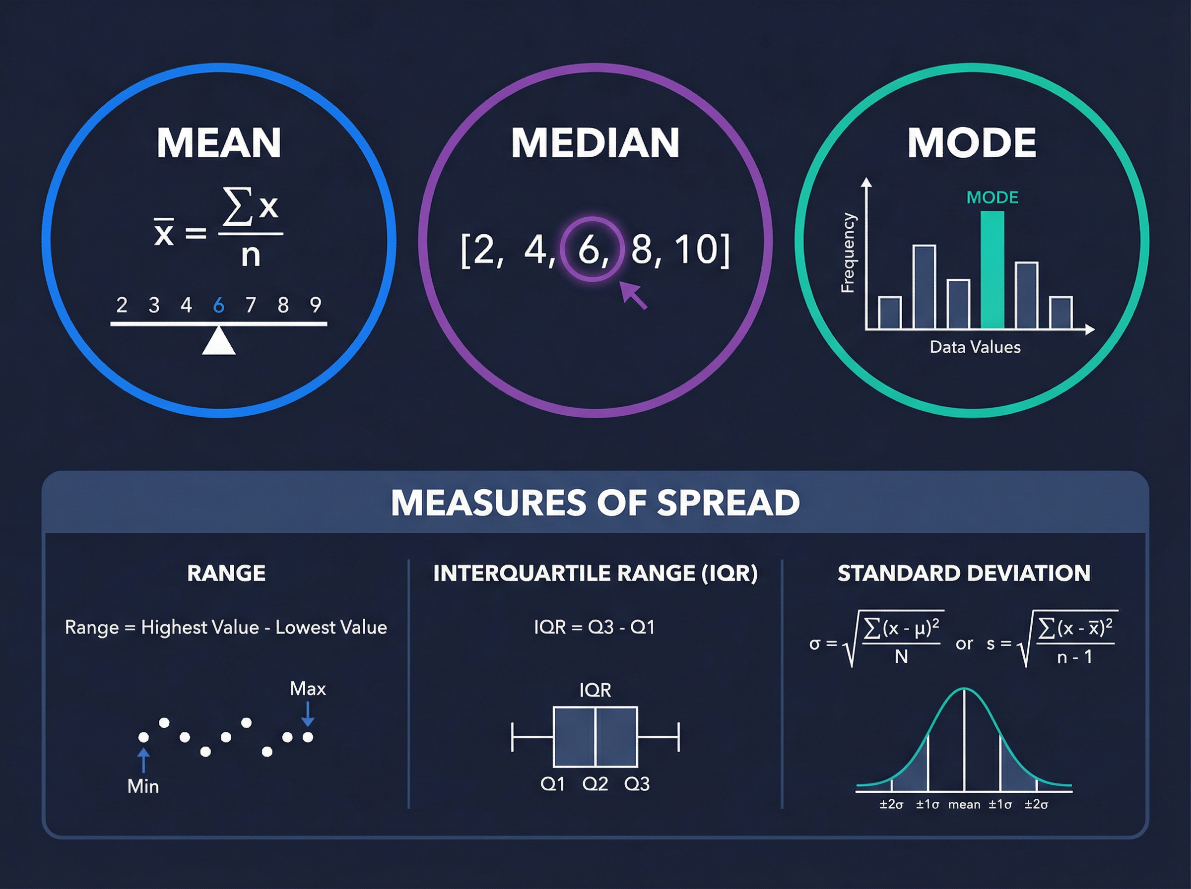
- Interquartile Range (IQR)
- The difference between the upper quartile and the lower quartile, representing the spread of the middle 50% of the data.
- Frequency Density
- The frequency divided by the class width, used as the y-axis on a histogram.
- Outlier
- An extreme value that lies significantly outside the overall pattern of the data.
Worked Examples
Worked Example
Question: The table shows information about the heights, $h$ cm, of 60 plants. Calculate an estimate for the mean height of the plants. (4 marks) | Height ($h$ cm) | Frequency | |---|---| | $10 < h \le 20$ | 8 | | $20 < h \le 30$ | 15 | | $30 < h \le 40$ | 24 | | $40 < h \le 50$ | 13 |
Solution: Step 1: Find the midpoint ($x$) of each class interval. - $10 < h \le 20$: Midpoint = 15 - $20 < h \le 30$: Midpoint = 25 - $30 < h \le 40$: Midpoint = 35 - $40 < h \le 50$: Midpoint = 45 Step 2: Multiply each midpoint by its frequency ($fx$). - $8 \times 15 = 120$ - $15 \times 25 = 375$ - $24 \times 35 = 840$ - $13 \times 45 = 585$ Step 3: Find the total sum of the frequencies ($\sum f$) and the total sum of $fx$ ($\sum fx$). - $\sum f = 8 + 15 + 24 + 13 = 60$ - $\sum fx = 120 + 375 + 840 + 585 = 1920$ Step 4: Divide $\sum fx$ by $\sum f$ to find the estimated mean. - Mean = $1920 \div 60 = 32$ Final answer: 32 cm
Worked Example
Question: A bag contains 5 red counters and 3 blue counters. A counter is taken at random from the bag and not replaced. A second counter is then taken. Calculate the probability that both counters are the same colour. (4 marks)
Solution: Step 1: Identify the two successful pathways: (Red, Red) OR (Blue, Blue). Step 2: Calculate the probability of (Red, Red). - P(First is Red) = 5/8 - P(Second is Red | First was Red) = 4/7 (one red removed, one counter total removed) - P(Red AND Red) = 5/8 × 4/7 = 20/56 Step 3: Calculate the probability of (Blue, Blue). - P(First is Blue) = 3/8 - P(Second is Blue | First was Blue) = 2/7 - P(Blue AND Blue) = 3/8 × 2/7 = 6/56 Step 4: Add the probabilities of the mutually exclusive pathways. - P(Same Colour) = P(Red, Red) + P(Blue, Blue) - P(Same Colour) = 20/56 + 6/56 = 26/56 Step 5: Simplify the fraction (optional unless specified, but good practice). - 26/56 = 13/28 Final answer: 13/28
Worked Example
Question: The incomplete histogram and table give information about the times, in minutes, taken by some students to complete a puzzle. Use the histogram to complete the table, and use the table to complete the histogram. (3 marks) | Time ($t$ minutes) | Frequency | |---|---| | $0 < t \le 10$ | 15 | | $10 < t \le 20$ | ? | | $20 < t \le 40$ | 16 | | $40 < t \le 50$ | ? |
Solution: Step 1: Use the known data to establish the scale on the histogram's y-axis (Frequency Density). - For $0 < t \le 10$: Frequency = 15, Class Width = 10. - Frequency Density (FD) = Frequency / Class Width = 15 / 10 = 1.5. - (Check the histogram to confirm the height of the first bar is 1.5). Step 2: Use the histogram to find the missing frequencies. - For $10 < t \le 20$: Read the FD from the histogram (e.g., FD = 2.5). Class width = 10. - Frequency = FD × Class Width = 2.5 × 10 = 25. - For $40 < t \le 50$: Read the FD from the histogram (e.g., FD = 0.8). Class width = 10. - Frequency = FD × Class Width = 0.8 × 10 = 8. Step 3: Use the table to complete the missing bar on the histogram. - For $20 < t \le 40$: Frequency = 16, Class Width = 20. - FD = Frequency / Class Width = 16 / 20 = 0.8. - Draw a bar from 20 to 40 with a height of 0.8. Final answer: Missing frequencies are 25 and 8. The bar for 20-40 is drawn at height 0.8.
Practice Questions
Question: A group of 20 students took a maths test. The median score was 65 and the interquartile range was 12. A second group of 20 students took the same test. Their median score was 72 and their interquartile range was 8. Compare the performance of the two groups. (2 marks)
Answer:
Question: A biased coin is flipped twice. The probability of getting a Head on any flip is 0.7. Calculate the probability of getting exactly one Head and one Tail. (3 marks)
Answer:
Question: The cumulative frequency graph shows the weights of 80 apples. The median weight is 120g, the lower quartile is 105g, and the upper quartile is 135g. The lightest apple is 90g and the heaviest is 160g. Draw a box plot to represent this data. (3 marks)
Answer:
Question: A factory produces lightbulbs. The probability that a lightbulb is defective is 0.02. A sample of 500 lightbulbs is tested. Calculate an estimate for the number of defective lightbulbs in the sample. (2 marks)
Answer:
Question: Explain why the median is a more appropriate average than the mean for a dataset of salaries in a company where the CEO earns £2,000,000 and the other 50 employees earn around £30,000. (1 mark)
Answer: