Probability — OCR GCSE Study Guide

## Overview  Probability is the mathematical language of uncertainty. In your GCSE Mathematics exam, it serves as a critical bridge between arithmetic (fractions, decimals, percentages) and real-world logic. Examiners use probability questions to test your ability to process information, apply logical steps, and handle fractions and decimals under pressure. Whether you are aiming for Foundation or Higher tier, probability is guaranteed to appear. It connects seamlessly to ratio, proportion, and algebra. Typical exam questions range from simple 1-mark recall questions (like placing an event on a probability scale) to complex 5-mark synoptic questions involving tree diagrams without replacement or algebraic probability.  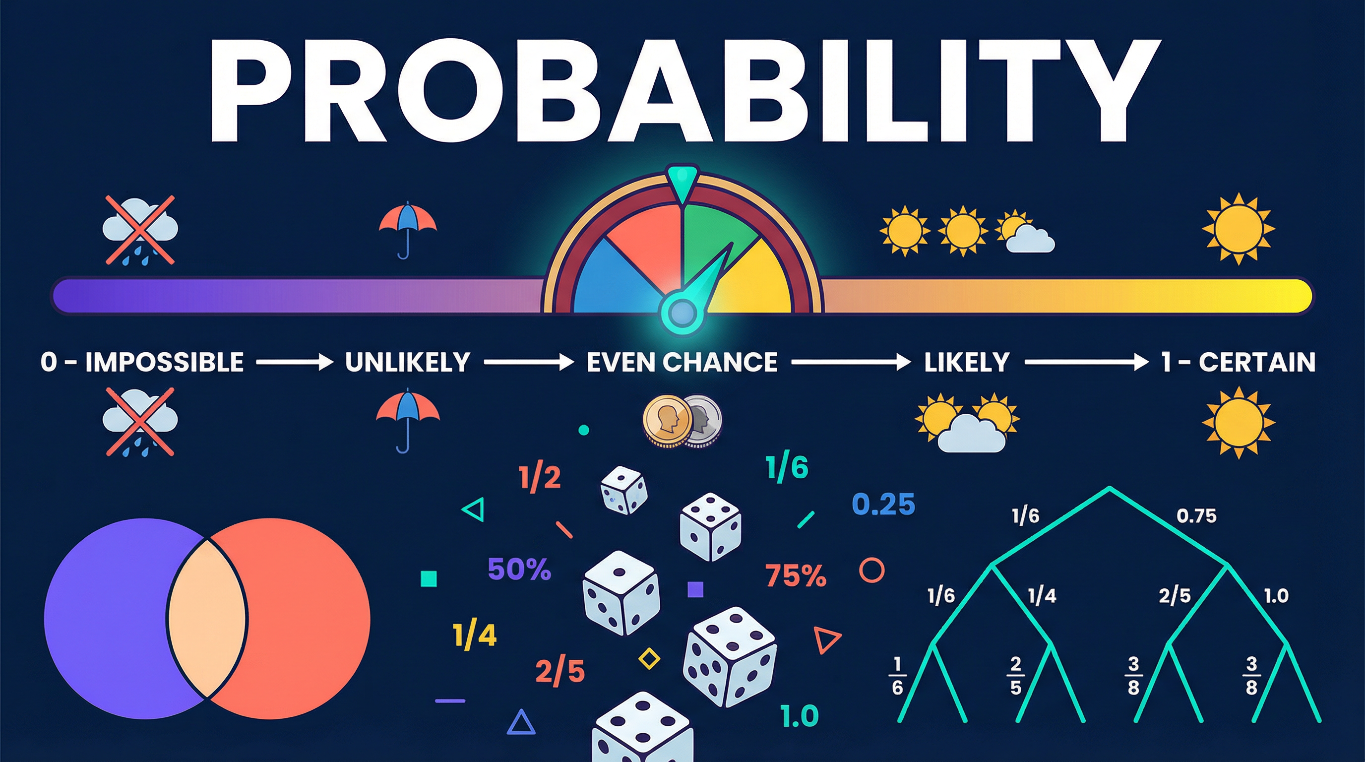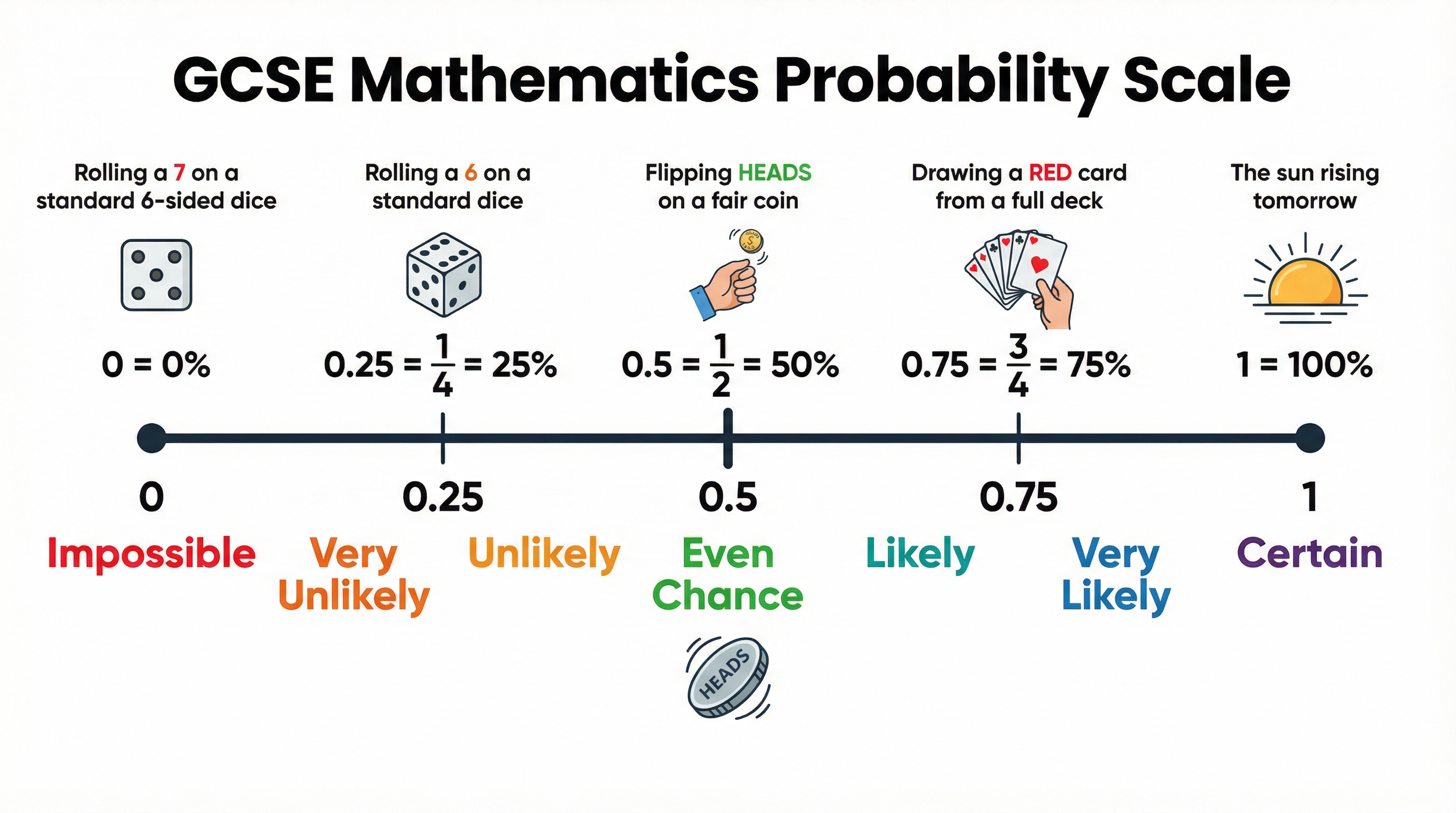## Key Concepts ### Concept 1: The Probability Scale and Basic Calculations Probability is always expressed as a number between $0$ (impossible) and $1$ (certain). You can write this as a fraction, a decimal, or a percentage. Examiners will award no marks if you write a probability greater than 1 or less than 0.  Theoretical probability is calculated when all outcomes are equally likely (like a fair dice or a fair coin). The formula is: $$P(\text{event}) = \frac{\text{Number of successful outcomes}}{\text{Total number of possible outcomes}}$$ **Example**: What is the probability of rolling a prime number on a standard 6-sided dice? The prime numbers are 2, 3, and 5. There are 3 successful outcomes out of 6 possible outcomes. $P(\text{prime}) = \frac{3}{6} = \frac{1}{2}$. ### Concept 2: The Exhaustive Rule (Adding to 1) One of the most frequently tested concepts is that the sum of the probabilities of all mutually exclusive exhaustive events is 1. This means if you know the probability of an event happening, you can find the probability of it *not* happening. $$P(\text{Not A}) = 1 - P(\text{A})$$ **Example**: If the probability of a train being late is $0.15$, the probability of it not being late is $1 - 0.15 = 0.85$. 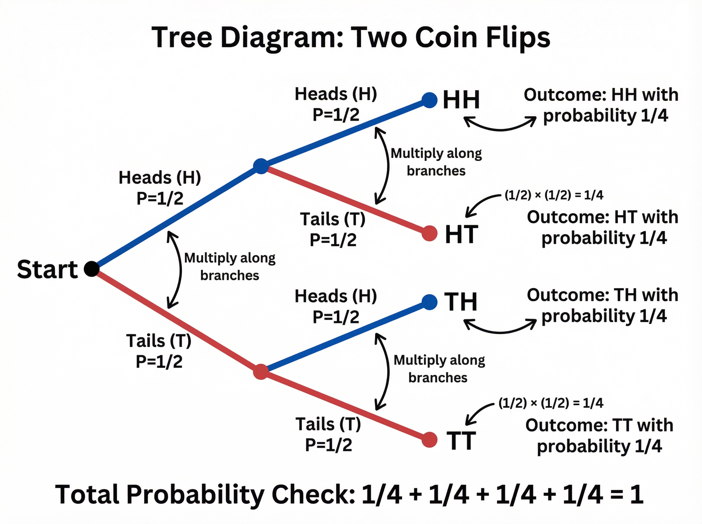### Concept 3: Tree Diagrams (Independent and Dependent Events) Tree diagrams are essential for visualising two or more events happening in sequence. They are heavily tested at both Foundation and Higher tiers.  - **Independent Events (With Replacement)**: The outcome of the first event does not affect the second. The denominator remains the same. - **Dependent Events (Without Replacement)**: The outcome of the first event *does* affect the second. If you remove an item without replacing it, the total number of items (the denominator) decreases by 1 for the second branch. The golden rules for tree diagrams: 1. **Multiply** along the branches to find the probability of a combined outcome (the "AND" rule). 2. **Add** the final probabilities if there is more than one way to achieve the desired result (the "OR" rule). 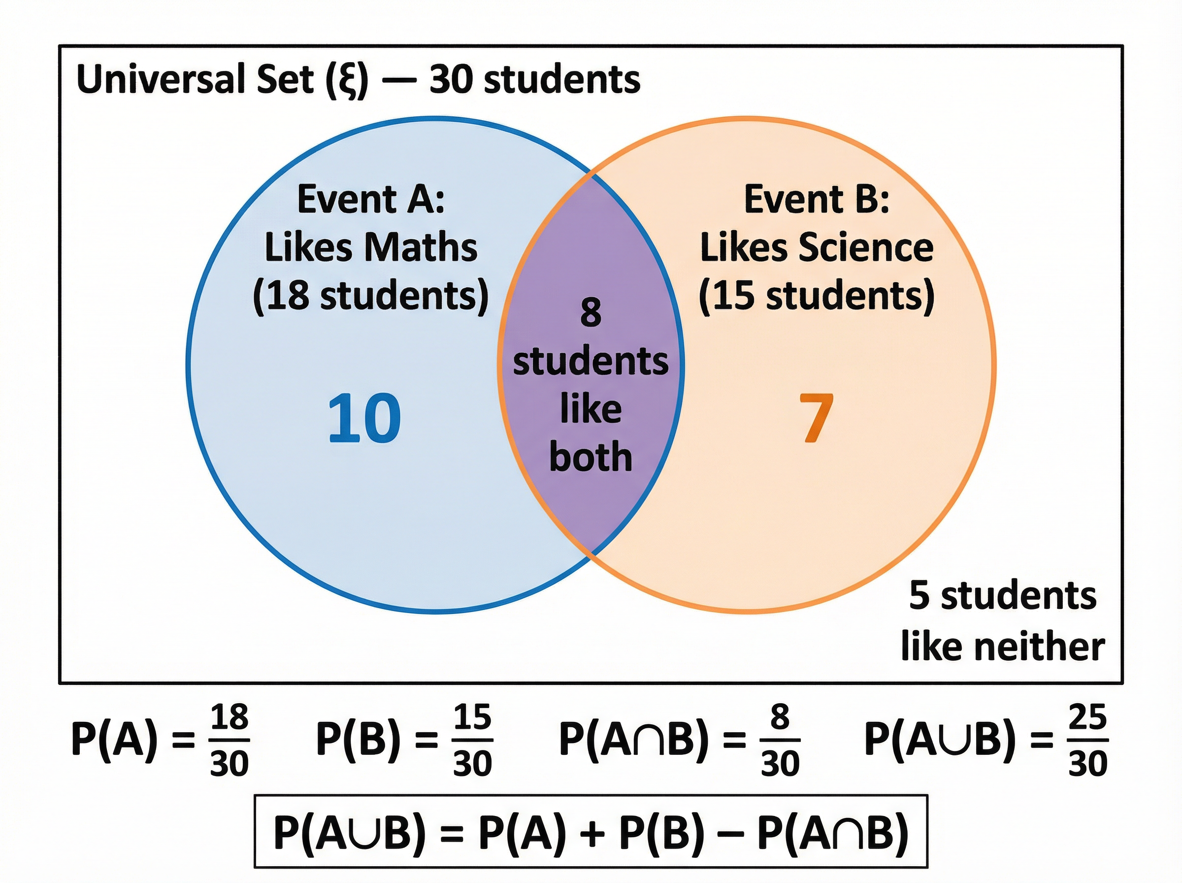### Concept 4: Venn Diagrams and Set Notation Venn diagrams are used to sort data and calculate probabilities involving overlapping categories. You must be comfortable with set notation: - $A \cup B$ (A union B): Items in A, or B, or both. - $A \cap B$ (A intersection B): Items in both A and B. - $A'$ (A prime/complement): Items not in A.  ### Concept 5: Relative Frequency (Experimental Probability) When we don't know the theoretical probability (e.g., if a dice might be biased), we conduct an experiment. The relative frequency is an estimate of the probability based on experimental data. $$\text{Relative Frequency} = \frac{\text{Number of successful trials}}{\text{Total number of trials}}$$ **Examiner Tip**: Examiners frequently ask how to make an estimate more reliable. The answer is always: "Increase the number of trials." ## Mathematical/Scientific Relationships - **Theoretical Probability**: $P(E) = \frac{\text{successful outcomes}}{\text{total outcomes}}$ - **Exhaustive Rule**: $P(A) + P(\text{Not A}) = 1$ - **Expected Frequency**: $\text{Expected Frequency} = \text{Probability} \times \text{Number of trials}$ - **Addition Rule (Mutually Exclusive)**: $P(A \text{ or } B) = P(A) + P(B)$ - **Multiplication Rule (Independent)**: $P(A \text{ and } B) = P(A) \times P(B)$ - **General Addition Rule**: $P(A \cup B) = P(A) + P(B) - P(A \cap B)$ ## Practical Applications Probability is used extensively in the real world: - **Insurance and Risk**: Actuaries calculate the probability of accidents to set insurance premiums. - **Quality Control**: Factories test a sample of products to estimate the probability of a defective item in the entire batch. - **Weather Forecasting**: Meteorologists use complex models to predict the probability of precipitation.