Subject: Mathematics | Level: GCSE | Exam Board: WJEC
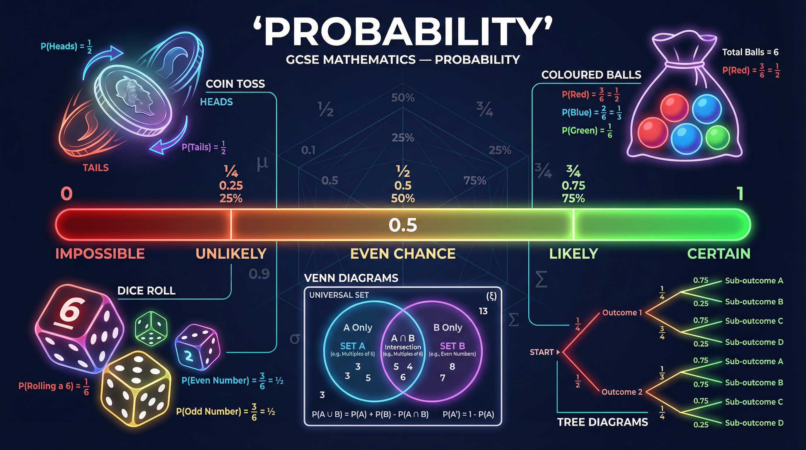
Mastering Probability is essential for securing high marks in your GCSE Mathematics exams. This guide covers everything from the basic probability scale and relative frequency to complex tree diagrams and Venn diagrams, ensuring you know exactly what examiners are looking for.
Revision Notes & Key Concepts
Key Terms & Definitions
- Mutually Exclusive
- Events that cannot happen at the same time. If A happens, B cannot happen.
- Independent Events
- Events where the outcome of one does not affect the probability of the other occurring.
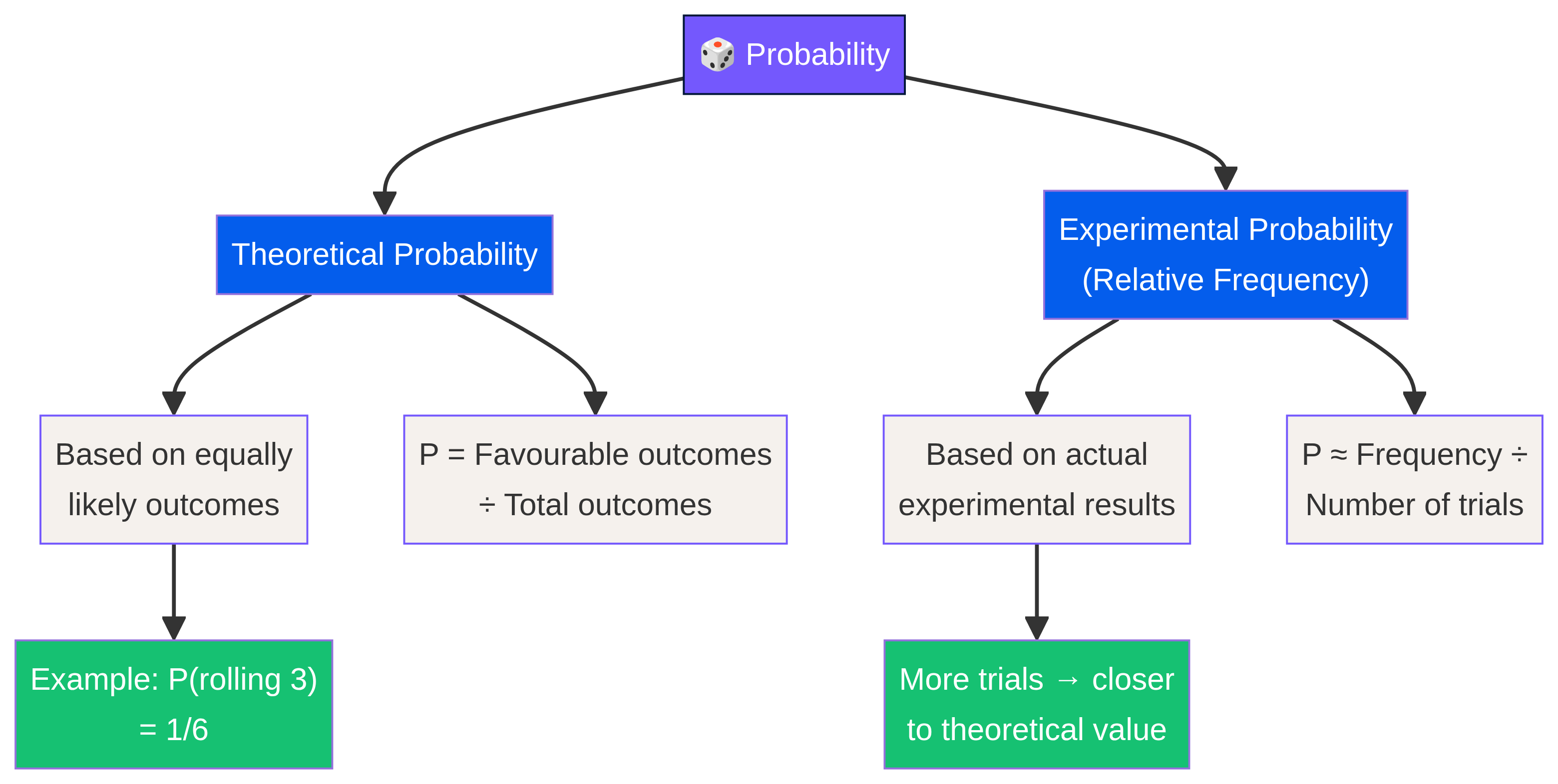
- Relative Frequency
- An estimate of probability based on the results of an experiment. Calculated as frequency of successful trials divided by total trials.
- Expected Frequency
- The theoretical number of times an event should occur over a given number of trials.
- Intersection
- The set of outcomes that belong to both event A and event B simultaneously.
- Sample Space
- The set of all possible outcomes of an experiment.
Worked Examples
Worked Example
Question: A biased spinner can land on 1, 2, 3 or 4. The table shows the probabilities of landing on 1, 2 and 3. The probability of landing on 4 is missing. Table: 1 (0.25), 2 (0.15), 3 (0.4), 4 (x). Work out the probability that the spinner lands on 4.
Solution: Step 1: The sum of all probabilities must equal 1. Step 2: Add the known probabilities: 0.25 + 0.15 + 0.4 = 0.8 Step 3: Subtract from 1 to find the missing probability: 1 - 0.8 = 0.2 Final answer: 0.2
Worked Example
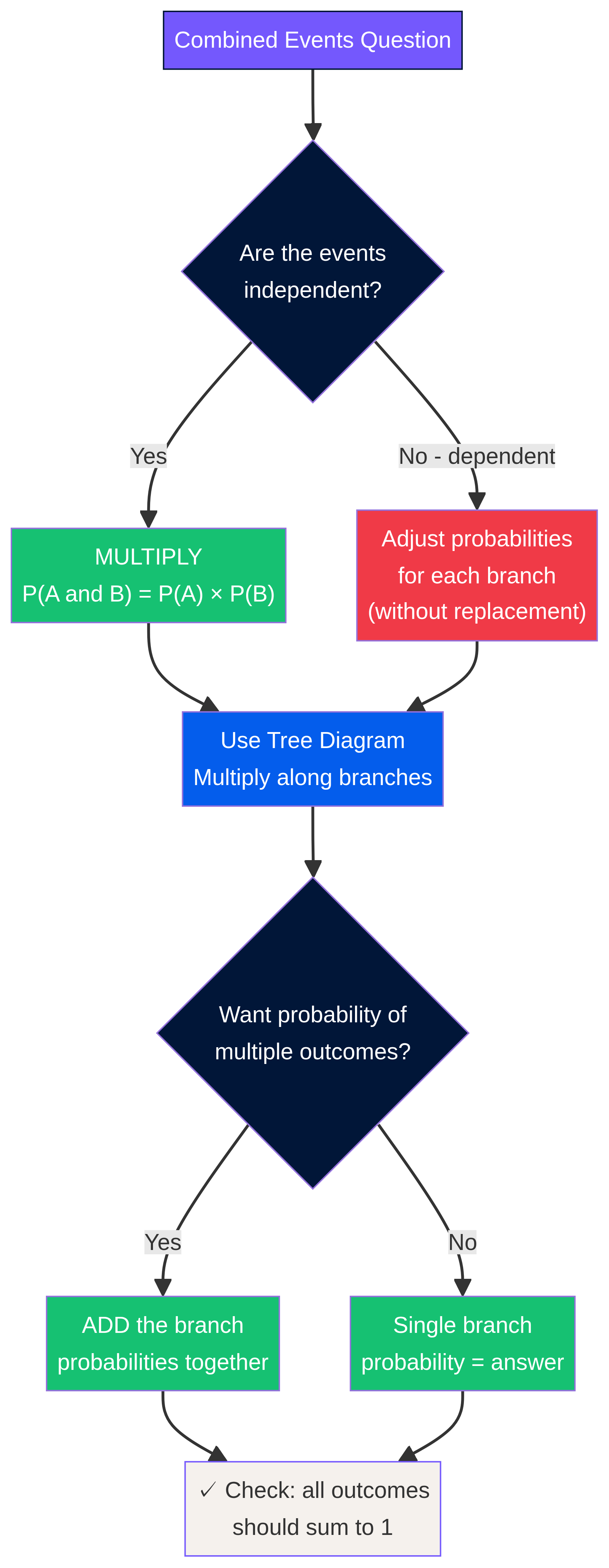
Question: A bag contains 5 red counters and 3 blue counters. A counter is taken at random from the bag and not replaced. A second counter is then taken at random from the bag. Calculate the probability that both counters are the same colour.
Solution: Step 1: Identify the successful outcomes: (Red, Red) or (Blue, Blue). Step 2: Calculate P(Red, Red). First pick is 5/8. Second pick is 4/7 (one red removed, one total removed). P(R,R) = 5/8 × 4/7 = 20/56. Step 3: Calculate P(Blue, Blue). First pick is 3/8. Second pick is 2/7. P(B,B) = 3/8 × 2/7 = 6/56. Step 4: Add the probabilities of the mutually exclusive outcomes. P(Same Colour) = 20/56 + 6/56 = 26/56. Final answer: 26/56 (or 13/28)
Worked Example
Question: In a class of 30 students, 18 study French (F), 14 study Spanish (S), and 5 study neither. Draw a Venn diagram to represent this information and use it to find the probability that a student chosen at random studies both French and Spanish.
Solution: Step 1: Find the number of students who study at least one language: 30 (total) - 5 (neither) = 25. Step 2: Find the intersection (both). If we add French and Spanish: 18 + 14 = 32. The difference between this and the number studying at least one language is the intersection: 32 - 25 = 7. So, 7 students study both. Step 3: Complete the Venn diagram. Intersection = 7. French only = 18 - 7 = 11. Spanish only = 14 - 7 = 7. Outside circles = 5. Check: 11 + 7 + 7 + 5 = 30. Step 4: Calculate the probability. Favourable outcomes (both) = 7. Total outcomes = 30. Final answer: 7/30
Practice Questions
Question: A fair ordinary dice is rolled once. Write down the probability that it lands on a number greater than 4.
Answer:
Question: The probability that a biased coin lands on heads is 0.6. The coin is flipped 150 times. Work out an estimate for the number of times the coin lands on heads.
Answer:
Question: A bag contains 7 red discs and 3 green discs. A disc is chosen at random, its colour noted, and then replaced. A second disc is then chosen. Calculate the probability that both discs are different colours.
Answer:
Question: There are 12 sweets in a box. 5 are lemon, 4 are strawberry, and 3 are orange. Sarah takes two sweets at random from the box without replacing the first one. Work out the probability that she takes exactly one strawberry sweet.
Answer:
Question: ξ = {integers from 1 to 10}. A = {prime numbers}. B = {odd numbers}. Draw a Venn diagram to represent this. A number is chosen at random from the universal set. Find the probability that the number is in the set A ∪ B.
Answer: