Study Notes
Overview
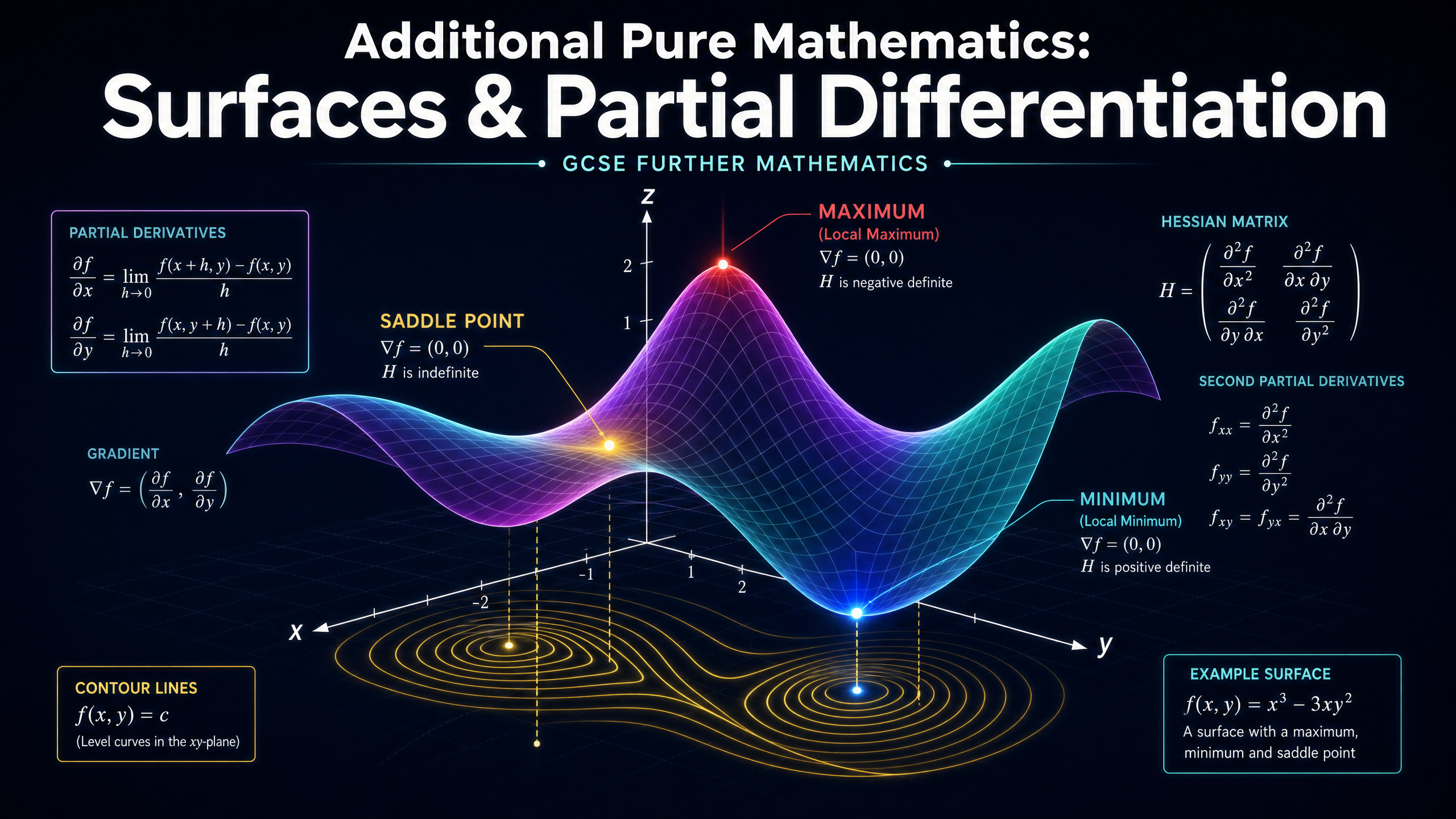
Welcome to Additional Pure Mathematics 2g: Surfaces and Partial Differentiation. In this topic, we extend the calculus you learned in 2D into the three-dimensional world. Instead of curves defined by y = f(x), we will analyse surfaces defined by z = f(x, y). This is a crucial area of Further Mathematics because it forms the foundation for advanced physics, engineering, and economics, where multiple variables interact simultaneously.
You will learn how to visualise these 3D surfaces using contour lines and cross-sections. More importantly, you will master partial differentiation — the technique of differentiating with respect to one variable while treating the other as a constant. This allows us to find the gradient of a surface in different directions. By setting these partial derivatives to zero, we can locate stationary points. Finally, you will use the Hessian matrix to classify these points as local maxima, local minima, or saddle points, and calculate the equation of the tangent plane touching the surface.
Examiners typically test this topic through multi-part questions: calculating partial derivatives, solving simultaneous equations to find coordinates, applying the Hessian test, and forming the tangent plane equation.
Key Concepts
Concept 1: Visualising 3D Surfaces
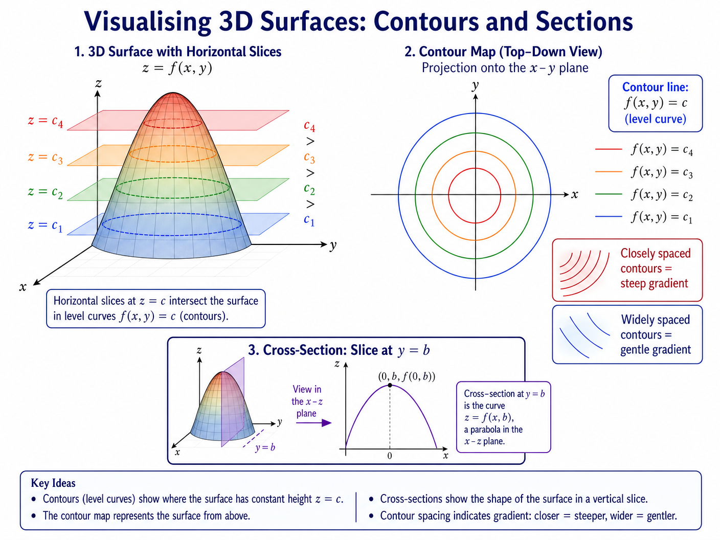
A function of two variables, z = f(x, y), represents a surface in 3D space. To understand its shape without complex 3D plotting, we use two main techniques:
- Contours (Level Curves): By setting z = c (a constant), we find the curve in the x-y plane where the surface has height c. This is exactly like contour lines on a geographical map. Closely spaced contours indicate a steep gradient, while widely spaced contours indicate a gentle slope.
- Cross-Sections: By fixing one variable (e.g., y = b), we take a vertical slice through the surface. The resulting curve z = f(x, b) shows the profile of the surface along that specific plane.
Concept 2: Partial Differentiation
When a function depends on both x and y, we can find its gradient in the x-direction by treating y as a constant and differentiating with respect to x. This is the partial derivative with respect to x, denoted as f_x or \frac{\partial f}{\partial x}.
Similarly, treating x as a constant and differentiating with respect to y gives the partial derivative with respect to y, denoted as f_y or \frac{\partial f}{\partial y}.
Example: Let f(x, y) = x^3y^2 + 4x - 5y.
- f_x = 3x^2y^2 + 4 (treating y as a constant)
- f_y = 2x^3y - 5 (treating x as a constant)
We can also find second partial derivatives:
- f_{xx} = \frac{\partial^2 f}{\partial x^2} (differentiate f_x with respect to x)
- f_{yy} = \frac{\partial^2 f}{\partial y^2} (differentiate f_y with respect to y)
- f_{xy} = \frac{\partial^2 f}{\partial x \partial y} (differentiate f_x with respect to y)
Crucial Rule: The Mixed Derivative Theorem states that for well-behaved functions, f_{xy} = f_{yx}. The order of differentiation does not matter.
Concept 3: Finding Stationary Points
A stationary point on a surface is where the tangent plane is perfectly horizontal. At this point, the gradient in both the x and y directions must be zero.
To find stationary points, we must solve the simultaneous equations:
f_x = 0 \quad \text{AND} \quad f_y = 0
Solving these gives the (x, y) coordinates of the stationary points. Substitute these back into z = f(x, y) to find the height z.
Concept 4: Classifying Stationary Points (The Hessian Test)
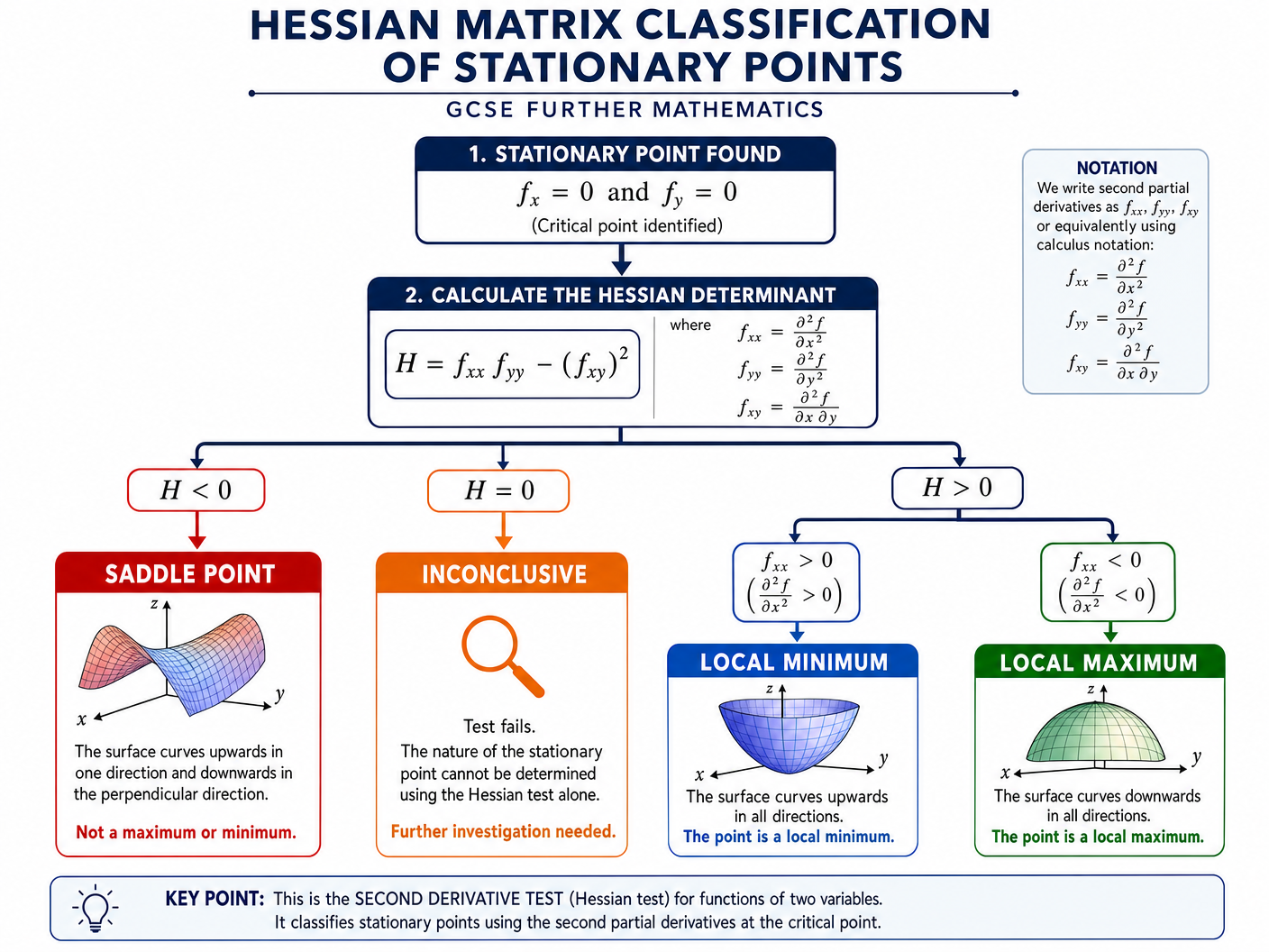
Once a stationary point is found, we classify it using the Hessian determinant, H:
H = f_{xx}f_{yy} - (f_{xy})^2
Evaluate H and f_{xx} at the stationary point (a, b):
- If H < 0: The point is a Saddle Point.
- If H > 0 AND f_{xx} > 0: The point is a Local Minimum.
- If H > 0 AND f_{xx} < 0: The point is a Local Maximum.
- If H = 0: The test is Inconclusive.
Concept 5: The Tangent Plane
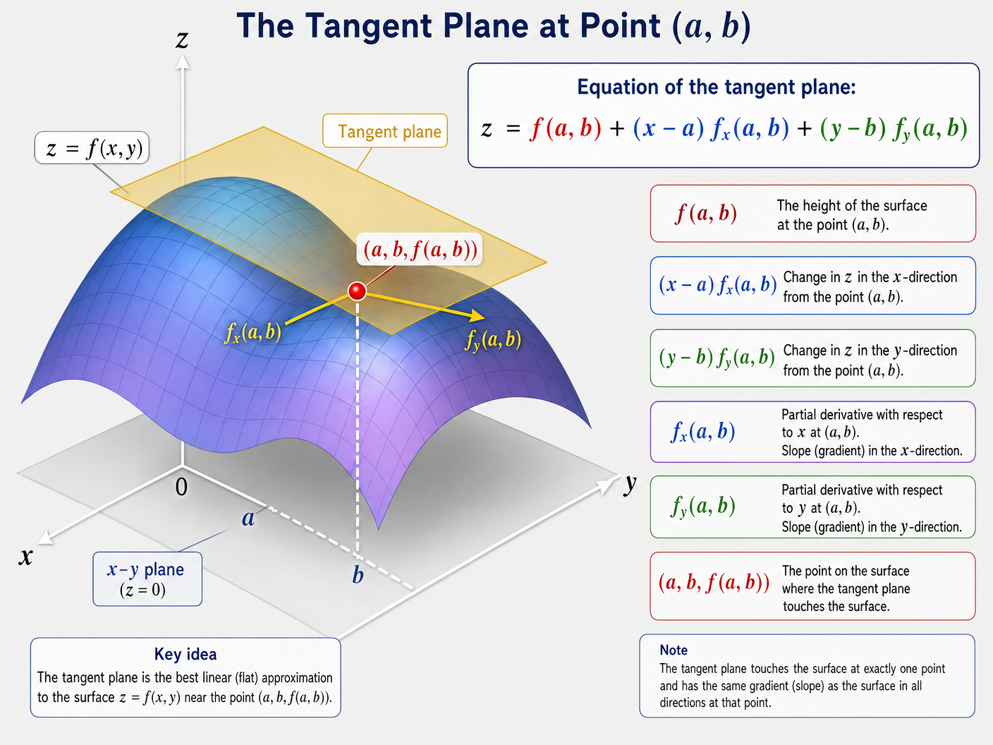
The tangent plane is the flat 2D plane that perfectly touches the surface at a specific point (a, b, f(a,b)). It is the 3D equivalent of a tangent line to a curve.
The equation of the tangent plane is given by:
z = f(a, b) + (x - a)f_x(a, b) + (y - b)f_y(a, b)
Podcast Episode
Listen to our 10-minute deep dive into surfaces, partial differentiation, and stationary points. Perfect for revising on the go!
Mathematical/Scientific Relationships
- Partial Derivative (x): f_x = \lim_{h \to 0} \frac{f(x+h, y) - f(x, y)}{h}
- Partial Derivative (y): f_y = \lim_{h \to 0} \frac{f(x, y+h) - f(x, y)}{h}
- Mixed Derivative Theorem: f_{xy} = f_{yx}
- Stationary Point Condition: f_x = 0 and f_y = 0
- Hessian Determinant: H = f_{xx}f_{yy} - (f_{xy})^2
- Tangent Plane Equation: z = f(a, b) + (x - a)f_x(a, b) + (y - b)f_y(a, b)
Practical Applications
- Machine Learning: Gradient descent algorithms use partial derivatives to find the minimum of complex loss functions (surfaces in multi-dimensional space) to train AI models.
- Economics: Profit maximisation for companies producing multiple products relies on finding the maximum stationary points of multi-variable profit functions.
- Physics & Engineering: Analysing stress, heat distribution, and fluid dynamics over surfaces requires partial differentiation.
Visual Resources
3 diagrams and illustrations
Interactive Diagrams
2 interactive diagrams to visualise key concepts
Conceptual Flow Outline
Flowchart: The process of finding and classifying stationary points.
Conceptual Flow Outline
Components required to form the tangent plane equation.
Worked Examples
4 detailed examples with solutions and examiner commentary
Practice Questions
Test your understanding — click to reveal model answers
Find the partial derivatives f_x and f_y of f(x, y) = 4x^3y^2 - 2x + 5y^3.
Hint: Remember to treat $y$ as a constant when finding $f_x$, and treat $x$ as a constant when finding $f_y$.
A surface has equation z = x^2 + 4xy + y^2 - 6x. Find the coordinates of the single stationary point.
Hint: Find $f_x$ and $f_y$, set them both to 0, and solve the resulting simultaneous equations.
Classify the stationary point (-1, 2) found in the previous question for the surface z = x^2 + 4xy + y^2 - 6x.
Hint: Calculate the second derivatives $f_{xx}, f_{yy}$, and $f_{xy}$. Then use the Hessian determinant formula.
Verify the Mixed Derivative Theorem for the function f(x, y) = x^3\sin(y) + e^{2x}y^2.
Hint: Calculate $f_{xy}$ and $f_{yx}$ separately and show they result in the exact same expression.
Find the equation of the tangent plane to the surface z = x^2\ln(y) at the point (3, 1, 0).
Hint: Find the partial derivatives, evaluate them at $x=3$ and $y=1$, and substitute into the tangent plane formula.