L: Data presentation and interpretation

Overview

AQA A-Level Mathematics 7357, section 3.13 L asks candidates to turn data into defensible conclusions. The calculations are usually short; the marks are often in the interpretation. You need to read a histogram by area, describe a scatter diagram precisely, choose statistics that represent the distribution fairly, and challenge data that may be misleading. This is the bridge between numerical technique and mathematical argument.

The topic can appear in the statistics content on Paper 2 or Paper 3. Each A-Level paper lasts 2 hours and is worth 100 marks, so a practical pacing guide is about 1.2 minutes per mark across the whole paper. There is no fixed number of marks for 3.13 L. A short one-mark interpretation, a linked multi-part context question, or a longer critique can all assess it. Calculators are permitted, but calculator output alone does not earn the communication marks: candidates must interpret it in context.

The four specification strands are: L1 single-variable diagrams and histogram area; L2 scatter diagrams, regression lines and correlation; L3 central tendency, variation and standard deviation; and L4 outliers, presentation choices and data cleaning. The same thinking connects directly to sampling, probability distributions and hypothesis testing.

Key concept 1: Histograms and single-variable data

A histogram displays continuous grouped data. Its bars touch because the values can lie anywhere within each class interval. The horizontal axis uses class boundaries, while the vertical axis is usually frequency density when class widths differ. A bar does not represent frequency through its height unless every class has the same width.

**Non-negotiable rule: frequency = bar area.**The relationship is:

• Frequency density = frequency ÷ class width. Must memorise.
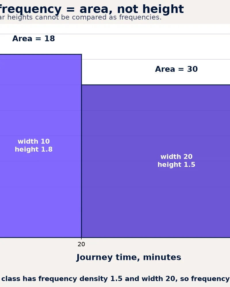
• Frequency = frequency density × class width. **Must memorise.**For example, a 20–40 minute class has width 20. If its frequency density is 1.5, its frequency is 1.5 × 20 = 30. A 10–20 minute class with height 2.5 also has frequency 2.5 × 10 = 25. Although the first bar is lower, it contains more observations because it is wider. Credit is given for calculating the area, not for comparing heights.

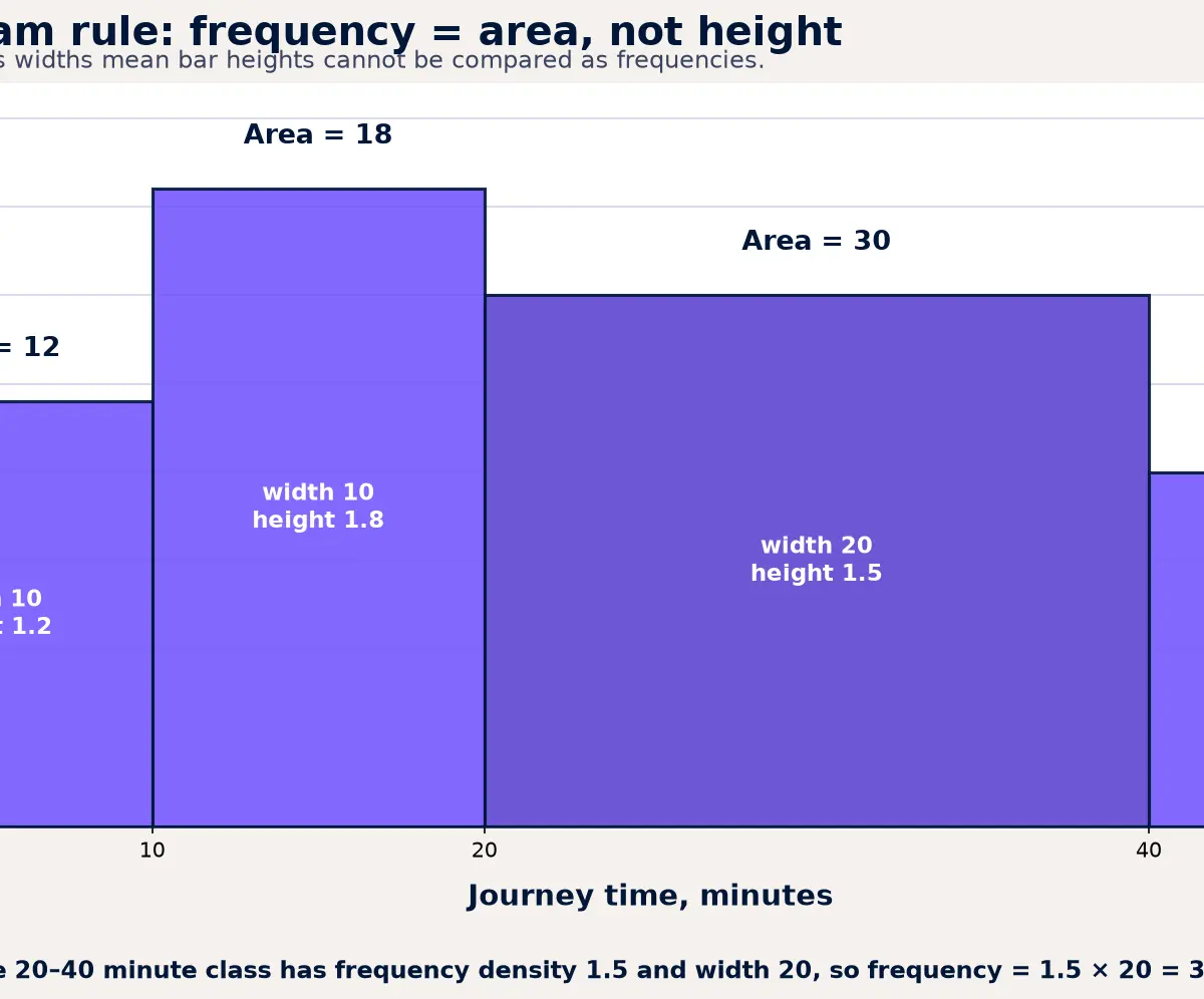
When interpreting a diagram, go beyond a bare observation. State the feature and what it means in context. Strong wording is: “Most journey times are between 10 and 30 minutes, while relatively few journeys exceed 40 minutes.” If the distribution has a long tail to large values, it is positively skewed; a long tail to small values is negatively skewed. A distribution can also be approximately symmetric, uniform, or bimodal. These shapes matter because they affect whether the mean is representative and whether a probability model may be appropriate later in the course.

Key concept 2: Bivariate data, correlation and regression

Bivariate data records two variables for each individual or unit, such as revision time and test score. A scatter diagram is the usual first view. For an interpretation question, train yourself to give D-F-S-C: Direction, Form, Strength, Context.

• Direction: positive, negative or no clear association.
• Form: linear, non-linear, clustered, or separate sections of the population.
• Strength: weak, moderate or strong, judged from how closely points follow the pattern.
• Context: name both variables rather than writing only “positive correlation”.

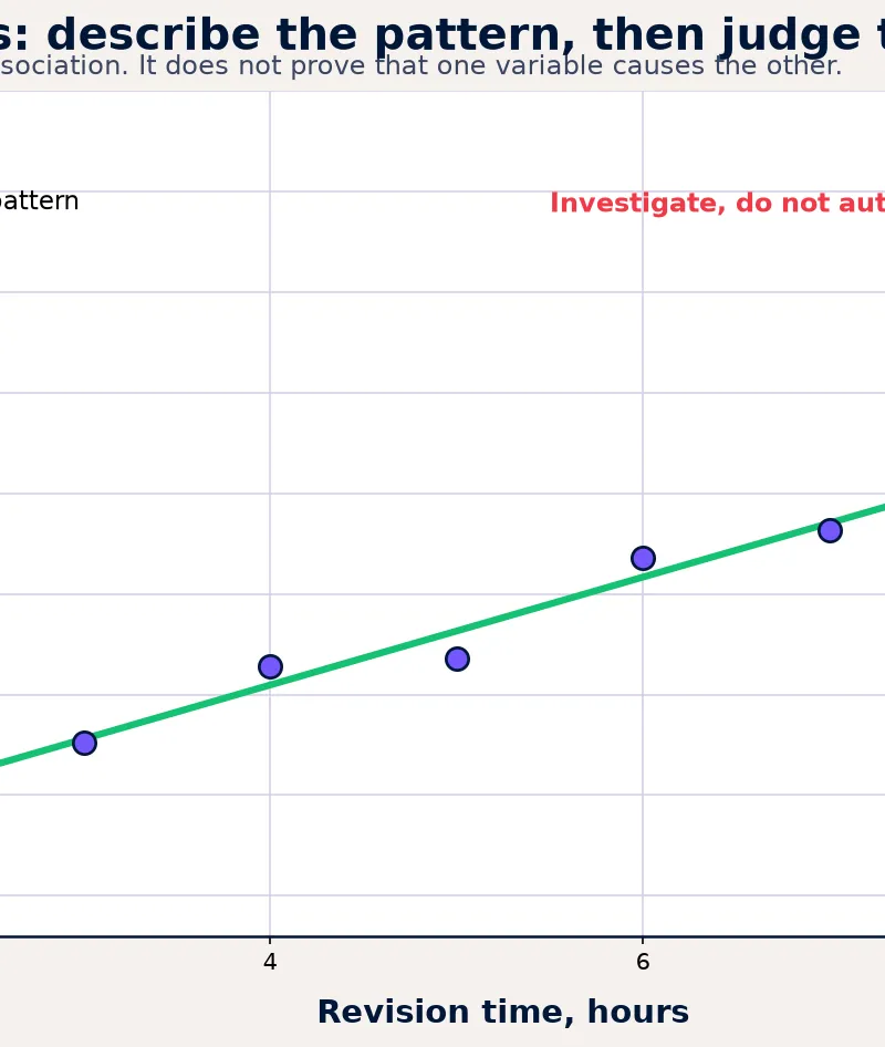
For example: “There is a moderately strong positive linear association between hours of revision and test score.” This is more precise than “the graph goes up”. If the points form two distinct clouds, candidates should say so. A single line may hide meaningful groups, for example results from two age groups or two measurement methods.

A regression line summarises the average linear trend. A point above the line has a y-value greater than the model predicts for its x-value; a point below has a lower y-value. Under AQA 3.13 L, calculations involving regression lines are excluded. The assessment is interpretation: judge whether the line is appropriate, recognise unusual points, and avoid extrapolating beyond the range of observed x-values.

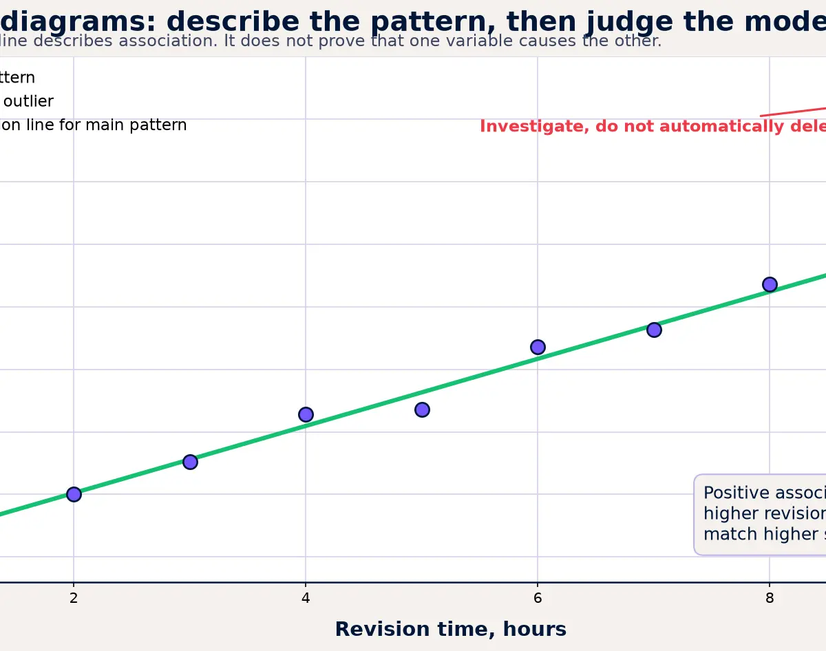
Most importantly, correlation does not imply causation. A positive association between ice-cream sales and rescue incidents does not show that ice cream causes the incidents. Temperature could be a third variable affecting both. In a response, a credible alternative explanation earns more than merely writing the slogan. Say what might be causing or influencing both variables, then state that the data alone cannot establish a causal relationship.

Key concept 3: Location, spread and standard deviation

A measure of central tendency describes a typical value. The mean uses every observation and is useful for reasonably symmetric data without influential extremes. The median is the middle ordered value and is more resistant to outliers and skew. The mode is the most frequent value and can be useful for categorical data. There is no automatic “best average”: select the statistic that serves the question.

Measures of variation show how spread out the data are. The range uses only two values, so one extreme value can alter it dramatically. The interquartile range describes the middle 50% and is more robust. The standard deviation measures typical distance from the mean: a small standard deviation means values are clustered, while a large one means they are dispersed.

Relevant relationships:

• x̄ = Σx ÷ n for the mean. Must memorise and understand.
• IQR = Q3 − Q1. Must memorise.
• s² = Σ(x − x̄)² ÷ n = Σx² ÷ n − x̄². Given on the AQA A-Level formula booklet.
• s = √(Σx² ÷ n − x̄²). **Given on the AQA A-Level formula booklet.**Here, n is the number of observations, Σx is the sum of the values, and Σx² means “square each value, then add”. It does not mean “add the values and then square”. When summary statistics are supplied, calculate the mean first, substitute carefully, keep full calculator precision, then give a sensible final accuracy. Marks are awarded both for a correct calculation and for an interpretation such as “Class B is more consistent because it has the smaller standard deviation.”

Calculator statistics mode is a time-saver, not a substitute for thinking. Clear a previous list, enter every datum accurately, select the appropriate standard-deviation output, and check whether the question wants a numerical answer, a comparison, or a conclusion in context.

Key concept 4: Outliers, data choice and data cleaning

A possible outlier is an observation unusually far from the general pattern. It may be a transcription error, a genuine rare observation, a value from a different population, or an important feature of the investigation. Never write “remove it” without a reason. Instead, investigate the source, units and context; decide whether the observation is plausible; state how including it changes the analysis; and report the limitation of the decision.

For a box plot, a common diagnostic is a value below Q1 − 1.5 × IQR or above Q3 + 1.5 × IQR. Must memorise if your class uses this convention. It is an investigation flag, not proof that a value is wrong. AQA requires recognition and interpretation of possible outliers, rather than blind deletion.

Data cleaning makes raw data fit for analysis while preserving an audit trail. Useful actions include:

1. Keep missing values visibly coded as missing, investigate them, or use a stated imputation method only when it is justified.
2. Check impossible values, wrong units, duplicated records and typing errors against the original source where possible.
3. Flag potential outliers and compare conclusions with and without them if that helps evaluate their influence.
4. Explain the consequence: removing data can reduce bias from an error, but can also introduce bias if genuine unusual cases are discarded.

Select the presentation to suit the variable and purpose. A bar chart is appropriate for categories; a histogram for continuous grouped data; a scatter diagram for two numerical variables; a box plot for comparing distribution and possible outliers. Critique a graph by considering labels, scale, class width, sample size, missing context and whether the display might exaggerate a difference.

Graph and data skills checklist

Before you answer, use this five-step routine:

1. Read the axes: variable, units, scale, class boundaries and whether the vertical axis is frequency or frequency density.
2. Calculate only what is needed: for a histogram, use area; for standard deviation, identify n, Σx and Σx².
3. Describe a visible feature: give direction, shape, cluster, spread or outlier.
4. Interpret in context: name the real variables and explain what the feature suggests.
5. Qualify the claim: recognise causation limits, extrapolation, sample limitations or data-quality concerns.

This routine is especially effective on AO2 and AO3 marks, where candidates must reason, communicate and evaluate rather than only carry out a routine procedure.

Exam technique and command words

For state or give, provide the requested statistic, label or conclusion directly. For describe, report distinct features of the display in context. For calculate, show the formula or the substitution, even when using a calculator, and give a suitably rounded answer. For explain, connect a feature to a consequence using “because”. For evaluate or critique, balance a strength against a limitation, then make a judgement relevant to the context.

A typical 4-mark histogram question often gives one mark for identifying a class width, one for a correct frequency-density relationship, one for accurate arithmetic, and one for a contextual interpretation. A 5- or 6-mark data question usually needs more than a calculation: expect marks for method, result, comparison, limitation and conclusion. Candidates lose marks when they write an unqualified causal claim, compare histogram heights with unequal widths, or report a standard deviation without saying what it shows.

Podcast companion

Use the ten-minute audio recap after completing the worked examples. Pause for the recall questions rather than letting the answer play straight away.