AQA · A-Level · Mathematics
Course version: 7357 · Version from Sept 2017
N: Statistical distributions
Statistical distributions turn uncertainty into marks: you decide whether a situation is Binomial or Normal, then use your calculator with defensible notation and clear interpretation. AQA rewards candidates who can challenge a weak model as confidently as they can calculate a probability, so this topic is about mathematical judgement as well as accuracy.
- 10 min read
- 4 worked examples
- 5 practice questions
- 8 key terms
Try the lesson
The start of the N: Statistical distributions lesson, made from checked teaching notes for this specification point.
Have a go first
The random variable X has the distribution B(10, 0.3). Find P(X = 3).
There is more to this lesson
The full lesson goes on to check your understanding and help you earn the marks. Create a free account to carry on, with your progress saved.
7 days Premium · Then the free plan continues · No card, no charge
Check what you remember
Read the wording for your board, then hide it and explain Random variable in your own words. Rough notes are fine. This is a self-check, with no mark or grade.
Reference: AQA
A variable whose numerical value is determined by the outcome of a random process.
Study Notes

Overview
AQA’s 3.15 N: Statistical distributions asks you to turn uncertain real-world situations into mathematical models. You must decide whether a variable is a count suited to a Binomial model, or a continuous measurement suited to a Normal model, then calculate and interpret probabilities accurately. The high-value skill is model choice: a calculator can produce a number, but candidates earn the explanation marks by stating why a model is, or is not, appropriate.
This topic sits at the centre of Paper 3. It connects directly to probability because every calculation describes an event, to data presentation because a histogram can support or challenge a Normal model, to sampling because poor sampling can make a model unrepresentative, and to hypothesis testing because a test statistic often uses a Binomial model. AQA’s specification is precise: N1 covers simple discrete distributions including Binomial, N2 covers Normal modelling and probabilities, and N3 requires justified model selection. Questions range from short calculator calculations to multi-step modelling explanations, usually worth 3–6 marks.
Examiner’s rule: a decimal answer is not a model. Write the distribution, translate the words into an event, calculate, then interpret in context.
Key Concepts
1. Random variables and the Binomial model
A random variableassigns a numerical value to each outcome. In this topic, it is often a count, such as the number of faulty items, late buses or successful shots. For a Binomial model, define the variable before using notation: “Let (X) be the number of components that fail.” Then write (X \sim B(n,p)), where (n) is the fixed number of trials and (p) is the probability of the chosen success on each trial.
Use the BINS test before you write (B(n,p)):
- Binary: each trial has exactly two outcomes, success or failure.
- Identical probability: (p) is constant from trial to trial.
- Number of trials: (n) is fixed in advance.
- Separate: the trials are independent.
For example, 20 independently manufactured components, each with probability 0.35 of failure, can be modelled by (X \sim B(20,0.35)). The wordfailure is simply the selected “success” for the model. It is the event being counted, so choose it deliberately.
Translate English into inequalities before pressing any calculator key. “Exactly 8” is (P(X=8)). “At most 8” is (P(X\leq8)). “At least 8” is (P(X\geq8)). “More than 8” is (P(X>8)), which is often entered using (1-P(X\leq8)). This line is frequently where candidates lose a method mark through an off-by-one boundary error.
A Binomial model can be unsuitable even if the variable is a count. Five cards drawn from a deck without replacement are not independent, because each draw changes the deck. The number of rainy days may not have a constant daily probability or independent outcomes. Do not write “not Binomial because it is unrealistic”. State the exact failed condition: for example, “the trials may not be independent because one traffic incident can delay several deliveries.”
2. The Normal distribution: centre, spread and area
$A Normal distribution models a continuous measurement with a smooth, symmetric bell-shaped pattern. Write (Y \sim N(\mu,\sigma^2)). The mean (\mu) fixes the centre. The standard deviation (\sigma) controls the spread. Crucially, the second parameter shown in the notation is the variance, (\sigma^2), whereas your calculator normally asks for the standard deviation, (\sigma).$
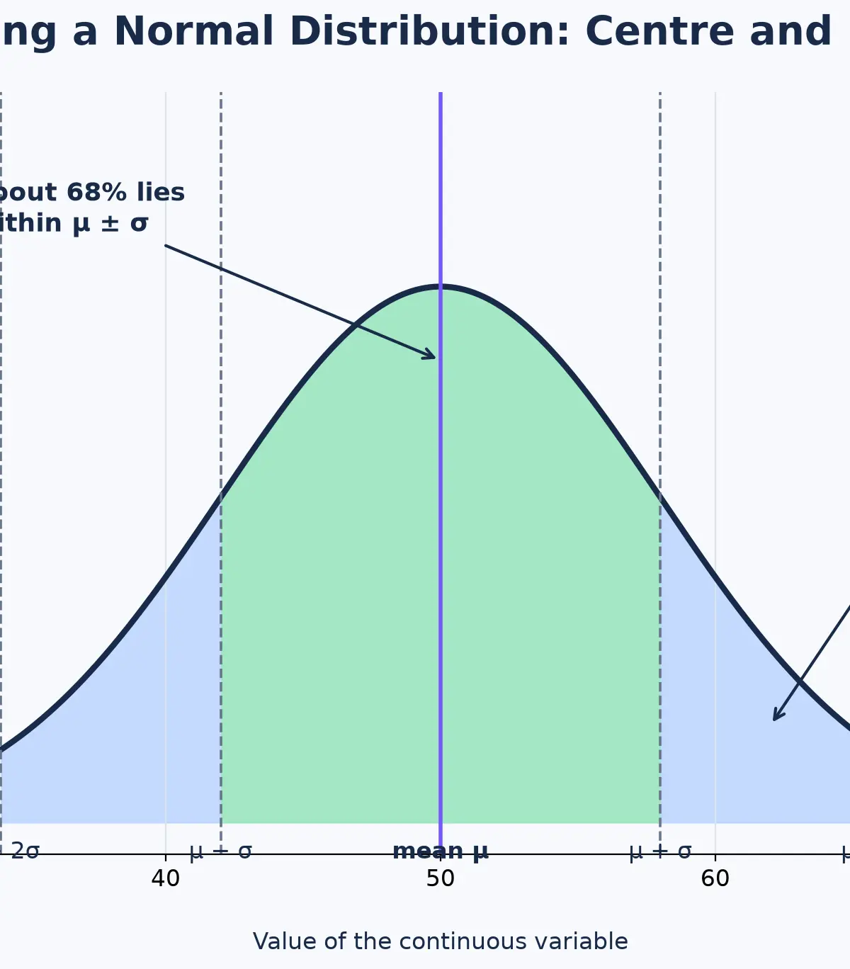
The total area under a Normal curve is 1, so an area is a probability. About 68% of values lie within one standard deviation of the mean, and about 95% lie within two standard deviations, provided the Normal model is appropriate. These are useful sense checks rather than replacements for a calculator calculation. If a 90th percentile is reported below the mean, for example, candidates should recognise that their tail or inverse-Normal entry is wrong.
A continuous model deals with intervals. (P(Y=180)=0) in the mathematical model, because a single point has no area. By contrast, (P(Y>180)) is the area to the right of 180. On a calculator, use NormalCD(lower, upper, μ, σ) for interval probabilities. Use a very large upper bound for “greater than”, and a very small lower bound for “less than”, following your calculator’s documented convention. Keep full calculator precision until the final answer.
For an inverse Normal question, the probability is known and the boundary is unknown. If (P(Y<k)=0.90), use InvNorm(0.90, μ, σ). Sketch the curve and shade the left 90% first. This tells you that (k) must be above the mean. The sketch is a 10-second check that can prevent a lost accuracy mark.
3. Choosing, justifying and rejecting a model
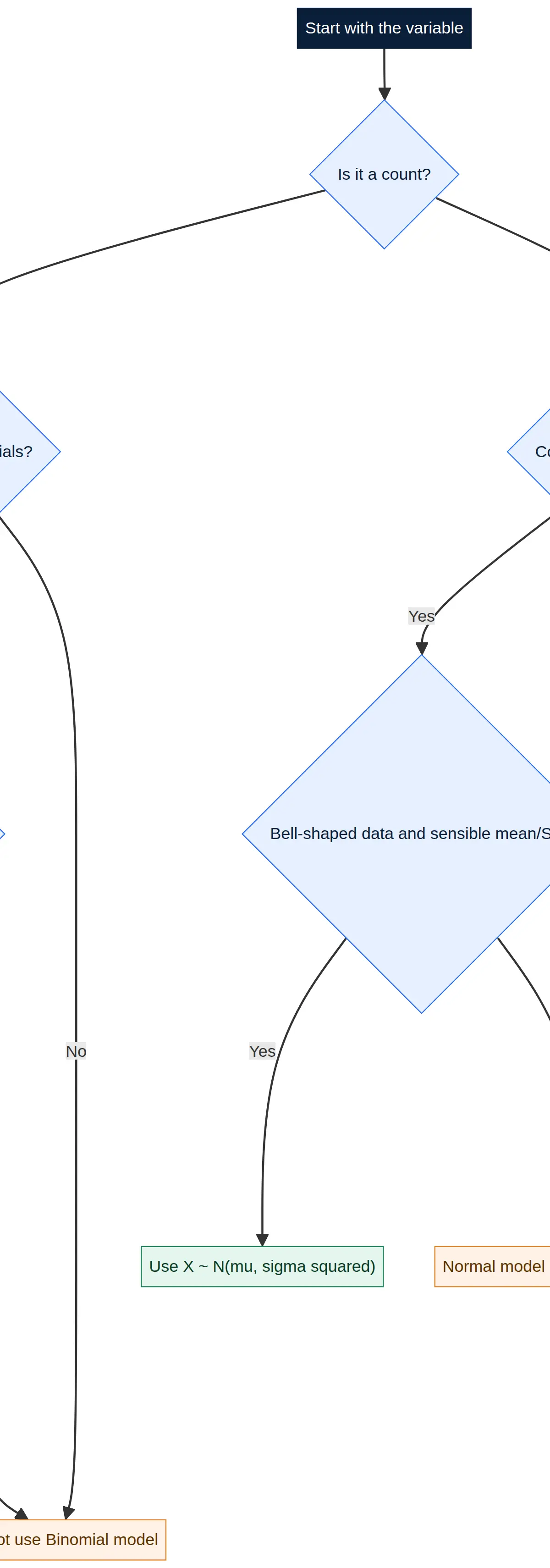
Start with the variable, not the calculator. A count of successes that meets BINS points to Binomial. A measured quantity that is continuous, plausibly symmetric and not constrained by an impossible tail may be modelled by Normal. A histogram is relevant evidence: one central peak with reasonably balanced sides supports a Normal model, while severe skewness, several peaks or a hard boundary close to the mean may make it weak.
A correct explanation uses data type plus assumptions. Strong: “A Normal model is plausible because journey time is continuous and the histogram is approximately symmetric and unimodal; however, negative values would be impossible, so the mean is sufficiently far above zero relative to the standard deviation.” Weak: “It is Normal because the graph is curved.” Strong: “A Binomial model is inappropriate because the components are sampled without replacement, so the probability of failure is not constant.” Weak: “It is not independent.” The latter does not explain why.
This is exactly the N3 skill. Credit is given for identifying the relevant condition and applying it to the context. If a question asks you to justify, do not provide only a probability. Build a sentence containing “because”.
4. Mathematical relationships and calculator routines
| Relationship | What it means | Formula-sheet status |
|---|---|---|
| (X\sim B(n,p)) | A Binomial random variable with fixed trial count (n) and success probability (p). | Must memorise notation and BINS conditions. |
| (P(X=r)=\binom{n}{r}p^r(1-p)^{n-r}) | Probability of exactly (r) successes. The combination counts the possible orders. | Must memorise/understand. In routine exam work, a calculator is normally used. |
| (Y\sim N(\mu,\sigma^2)) | A Normal variable with mean (\mu), variance (\sigma^2) and standard deviation (\sigma). | Must memorise notation. |
| (\sigma=\sqrt{\sigma^2}) | Convert variance in the model notation to the standard deviation required by the calculator. | Must memorise. |
| (z=\frac{x-\mu}{\sigma}) | Standardises a value by measuring its distance from the mean in standard deviations. | Must memorise. |
| (P(a<Y<b)=P(Y<b)-P(Y\leq a)) | An interval is the area between two boundaries. NormalCD calculates this directly. | Must memorise as a probability relationship. |
AQA’s formulae appendix states that required formulae and identities must be used without being supplied. Do not rely on a formula booklet to rescue the notation, the standardisation relationship or the Binomial conditions. You may use a calculator in the examination, but calculator syntax varies. Practise three functions on your own approved calculator: Binomial probability, Binomial cumulative distribution, and Normal/Inverse Normal distribution.
5. Graph and data skills
For a Normal curve, label the horizontal axis with the variable and units where given. Mark (\mu) at the centre and use equally spaced positions for (\mu\pm\sigma) and (\mu\pm2\sigma). Shade the required region, not the decorative whole curve. A right-tail probability has shading to the right; a percentile question has a boundary positioned so that the stated cumulative area is on the correct side.
When reading a histogram, distinguish frequency density from frequency. A bell-shaped outline supports, but does not prove, a Normal model. You should also consider whether the quantity is continuous, whether values can be negative, whether there are outliers and whether the sampling method makes the data representative. AQA links Normal distributions to histograms, mean, standard deviation, points of inflection and the Binomial distribution, so expect context-rich questions rather than isolated button pressing.
6. Practical applications and model limitations
Binomial models appear in quality assurance, clinical trial outcomes, marketing response rates and sport: each context counts whether a specified event happened. Normal models appear in manufacturing tolerances, heights, measured completion times and instrument error. A model is useful because it replaces many observations with a manageable structure, but it is always an approximation. The exam question may deliberately include a flaw, such as linked family responses, changing weather conditions or an impossible negative time. Spotting that flaw is a mathematical skill, not an optional comment.
7. Exam-ready response templates
For a Binomial calculation, a compact full-mark opening is: “Let (X) be the number of [successes]. Since there are (n) fixed independent trials, each with two outcomes and constant probability (p), (X\sim B(n,p)). Therefore (P(\text{event})=\ldots).” Use only the conditions supported by the question, but make the event visible before your calculator output. For a Normal calculation, write: “(Y\sim N(\mu,\sigma^2)). Hence (P(\text{interval or tail})=\ldots), so the estimated probability/proportion is (\ldots).”
For a model judgement, use a balanced frame: “The model is [appropriate / not appropriate] because [condition] is [met / not met] in this context. In particular, [specific contextual reason].” If evidence is incomplete, use qualified language such as “may not be appropriate” rather than claiming certainty. Examiners credit precise mathematics, not overconfident speculation. This wording is especially useful when a question gives a histogram, a sampling method or a practical limitation and asks you to explain rather than calculate.
Audio recap
Use the 10-minute audio recap after completing questions, then immediately attempt the retrieval prompts below without looking at the guide. Passive listening helps familiarity; retrieval is what secures marks.
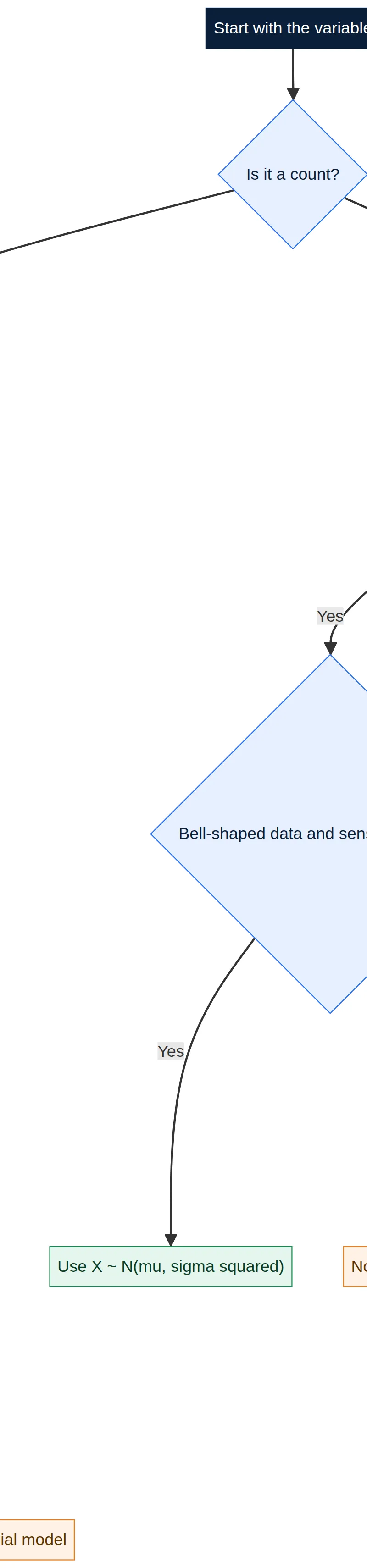
Interactive Diagrams
2 interactive diagrams to visualise key concepts
Conceptual Flow Outline
Use variable type and assumptions, not calculator availability, to select the model.
Conceptual Flow Outline
A calculator workflow that preserves both method marks and accuracy marks.
Worked Examples
4 worked examples — open one to explore the question and available guidance.
Practice Questions
Try the question, then reveal an answer plan or example response
A marketing email is opened independently by each recipient with probability 0.4. Of 12 recipients, calculate the probability that at most 3 open the email. [3 marks]
Hint: Define X as the number who open the email. ‘At most’ includes 3.
A bulb fails during testing with probability 0.2, independently of other bulbs. 15 bulbs are tested. Calculate the probability that more than 3 fail. [4 marks]
Hint: ‘More than 3’ is X > 3. A complement may be the easiest calculator route.
Scores S are modelled by S ~ N(68, 5²). Calculate P(62 < S < 74). [4 marks]
Hint: This is the area between two boundaries, not a probability at one point.
The lifetime L of a battery is modelled by L ~ N(40, 6²), in hours. Find q such that P(L < q) = 0.25. [4 marks]
Hint: The 25th percentile is below the mean. Use inverse Normal, not NormalCD.
A shop samples 5 products without replacement from a delivery of 30, records whether each is damaged and considers X, the number damaged. Evaluate whether X can be modelled by a Binomial distribution. [4 marks]
Hint: Some Binomial conditions hold. Identify the one altered by sampling without replacement.
Exam technique
How to turn what you know into marks
How to approach the question
Underline the variable and command word. Define the random variable, apply BINS or Normal-model evidence, state the distribution, translate the wording into a symbolic event, use the calculator, then write one sentence that answers the context. Sketch the Normal tail or percentile before entering calculator bounds.
How to structure your answer
For 3–4 calculation marks: model/event statement; correct calculator method; accurate value; interpretation if requested. For 4–6 justification marks: name the model, identify each relevant condition, apply it to the data, then reach a qualified conclusion. Use ‘because’ to connect every assertion to evidence.
Timing
Paper 3 is 120 minutes for 100 marks, so plan about 1.2 minutes per mark. A 4-mark distributions calculation should normally take 4–5 minutes, including notation and a brief check.
Common pitfalls
- Using P(X > 8) for ‘at least 8’. Write ≥, >, ≤ or = before using the calculator.
- Entering σ² as the calculator standard deviation. In N(μ, σ²), take the square root if the value supplied is a variance.
- Treating a count as automatically Binomial. Check all BINS conditions, especially independence and constant probability.
- Giving a Normal probability for an exact continuous value. Shade and calculate an interval or tail, not a point.
- Rounding a cumulative probability before using it in a later step. Keep the stored calculator value until the final reported answer.
What the command words want
- Compare
- Refer to both models or distributions using the same criteria: variable type, parameter values, spread, assumptions and the resulting probabilities.
- Explain
- Use a ‘because’ sentence that links a Binomial condition or Normal-model feature to the exact context.
- Describe
- Identify the visible shape, centre, spread or tail using mathematically correct vocabulary such as symmetric, skewed, discrete or continuous.
- Evaluate
- Give supporting evidence and limitations, then make a qualified judgement. A model can be useful without being perfect.
- Calculate
- Show the model and symbolic event, use a correct calculator function, retain accuracy, then state the answer to sensible precision with units where relevant.
- State/Give
- Write the precise distribution, parameter, probability or value required. Do not add an unsupported explanation.
Watch or listen (optional)
Test your understanding of N: Statistical distributions
Active recall beats re-reading. Take an instant quiz now to test what you’ve learned and lock it into long-term memory.
7 days Premium · Then the free plan continues · No card, no charge