AQA · A-Level · Mathematics
Course version: 7357 · Version from Sept 2017
O: Statistical hypothesis testing
Statistical hypothesis testing is where AQA candidates turn a sample result into a justified decision about a population. Master the fixed structure of hypotheses, tail, model, probability boundary and contextual conclusion, and you can secure method marks even before the final calculation.
- 9 min read
- 3 worked examples
- 5 practice questions
- 10 key terms
Try the lesson
The start of the O: Statistical hypothesis testing lesson, made from checked teaching notes for this specification point.
Have a go first
A random sample of 16 observations is taken from a Normal distribution with standard deviation 5. The sample mean is 52. A test is carried out at the 5% significance level with H₀: μ = 50 against H₁: μ > 50. Using the test statistic z = (x̄ − μ₀)/(σ/√n), decide whether H₀ should be rejected.
There is more to this lesson
The full lesson goes on to check your understanding and help you earn the marks. Create a free account to carry on, with your progress saved.
7 days Premium · Then the free plan continues · No card, no charge
Check what you remember
Read the wording for your board, then hide it and explain Null hypothesis (H₀) in your own words. Rough notes are fine. This is a self-check, with no mark or grade.
Reference: AQA
The initial statement about a population parameter that is assumed true when calculating the test probability; it contains an equality.
Study Notes

Overview
AQA A-Level Mathematics 7357, 3.16 O: Statistical hypothesis testing asks candidates to make a cautious inference about a population from sample data. You start with a claim, model what should happen if that claim is true, then decide whether the observed sample is too unusual to explain by chance. This is not a test of whether a claim is “proved”. It is a rule for deciding whether the evidence is strong enough to reject a null hypothesis at a stated significance level.
For AQA, the tested settings are a proportion in a binomial distribution, the mean of a Normal distribution when the variance is known, given or assumed, and interpretation of a supplied correlation coefficient using a p-value or critical value. Calculation of a correlation coefficient is excluded from this section. Hypothesis testing sits in Paper 3, which is a 2-hour, 100-mark paper. Expect short calculations and multi-step questions where the final contextual sentence earns a separate mark. 1 2
The subject becomes much easier when you see its fixed logic: claim → tail → model → probability boundary → contextual decision. Every answer should make that logic visible.
Key concept 1: hypotheses, tails and significance
The null hypothesis, written H₀, is the starting population claim. It must contain an equality, for example H₀: p = 0.20 or H₀: μ = 65. The alternative hypothesis, H₁, says what the question is investigating. Its inequality chooses the tail:
- H₁: parameter > stated value gives an upper-tail test.
- H₁: parameter < stated value gives a lower-tail test.
- H₁: parameter ≠ stated value gives a two-tail test.
The significance level, α, controls the risk of a false rejection. At α = 0.05, the procedure has at most a 5% probability of rejecting H₀ when H₀ is actually true. Credit is given for this exact idea. It does not mean “there is a 5% probability that H₀ is true”.
A critical region is the set of sample values so extreme that H₀ is rejected. The acceptance region contains values not extreme enough to reject H₀. In a p-value approach, calculate the probability of a result at least as extreme as the observed result, in the direction specified by H₁. Reject H₀ when p ≤ α. If p > α, write do not reject H₀. Candidates should never write “accept H₀”, because a non-significant sample has not proved the claim true.
Memory hook: CDDDC. Claim, Direction, Distribution, Decision, Context. If one of these is absent, an examiner can normally see exactly where marks have been lost.
Key concept 2: binomial tests for a proportion
Use a binomial test when the random variable counts successes in a fixed number of independent trials, with a constant probability of success under H₀. Define the random variable before using the calculator: “Let X be the number of successes in n trials.” Under H₀, write X ∼ B(n, p₀). This line is a common method mark because it links the population claim to the probability model.
For an upper-tail test, find the smallest integer c for which P(X ≥ c) ≤ α. The critical region is X ≥ c. For a lower-tail test, find the largest integer c for which P(X ≤ c) ≤ α. A two-tail test normally allocates α/2 to each tail. Because X is discrete, the actual probability in the chosen critical region may be less than α. That is correct. Do not move the boundary merely because the probability is not exactly 0.05.
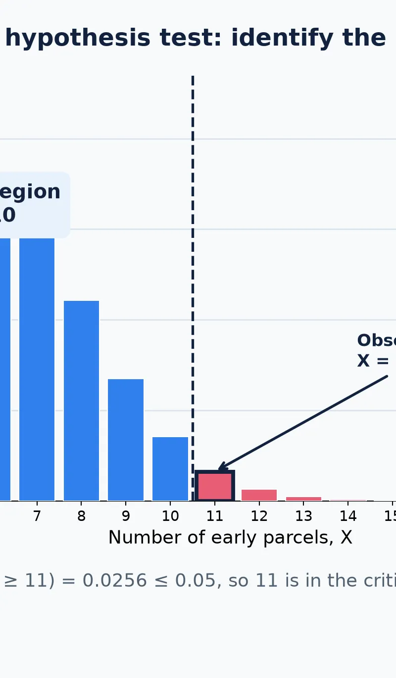
Suppose H₀: p = 0.20 and H₁: p > 0.20, with n = 30 and observed X = 11. Under H₀, X ∼ B(30, 0.20). The smallest upper critical value is 11 because P(X ≥ 11) = 0.0256, while P(X ≥ 10) = 0.0611. Therefore the critical region is X ≥ 11 and the observed result is significant at the 5% level.
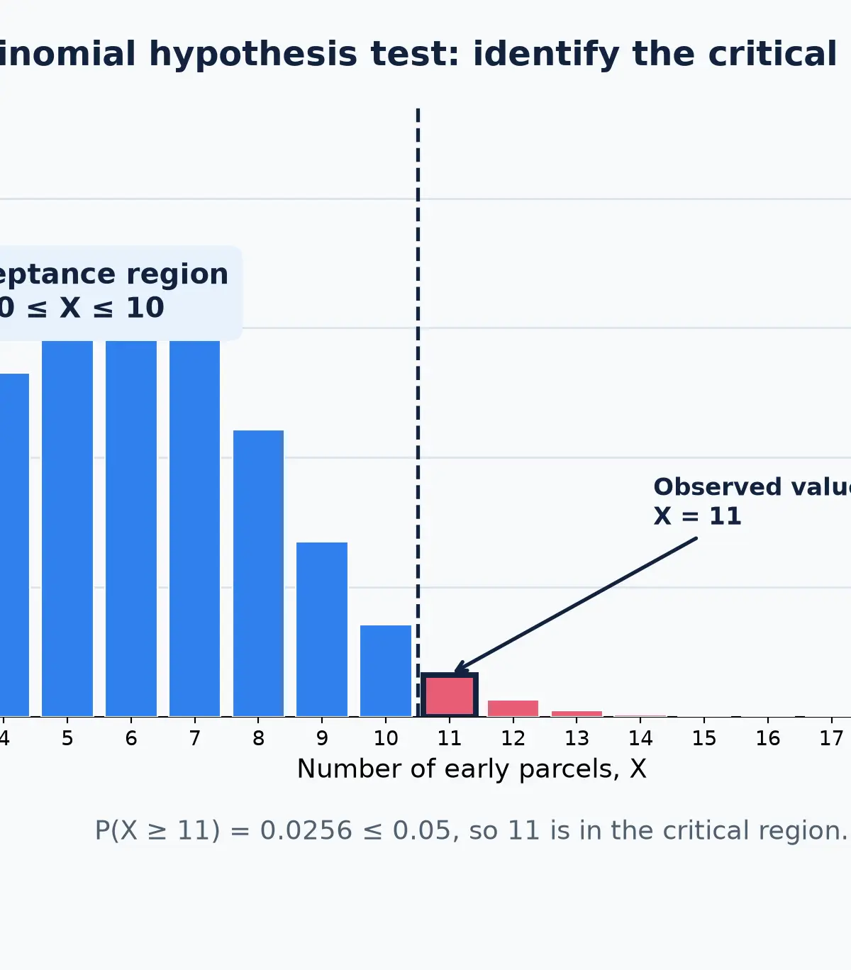
Why does this work? If p really were 0.20, large values of X would be rare. Seeing a value in the critical region is evidence against that model. It is not proof that a different value of p has been measured exactly.
Key concept 3: Normal tests for a population mean
Use this model only when the population is Normal and its variance is known, given or explicitly assumed. This condition is in the AQA specification. If the population variance is σ² and a sample of size n has mean x̄, then under H₀: μ = μ₀:
x̄ ∼ N(μ₀, σ²/n)
The standard error is σ/√n. Standardising gives z = (x̄ − μ₀)/(σ/√n). Compare z with the appropriate standard Normal critical value, or find the p-value. For a 5% upper-tail test, reject when z > 1.645. For a 5% two-tail test, reject when |z| > 1.960.
Example: a machine claims μ = 65 g, σ = 12 g and n = 36. A sample has x̄ = 68.5 g. For H₁: μ > 65:
z = (68.5 − 65)/(12/√36) = 1.75.
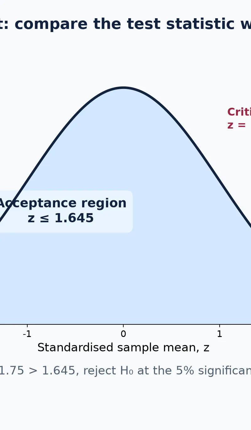
Since 1.75 > 1.645, reject H₀ at the 5% significance level. The contextual conclusion is: “There is sufficient evidence that the mean carton mass is greater than 65 g.” A bare sentence such as “significant” is incomplete, because it does not answer the claim in the question.
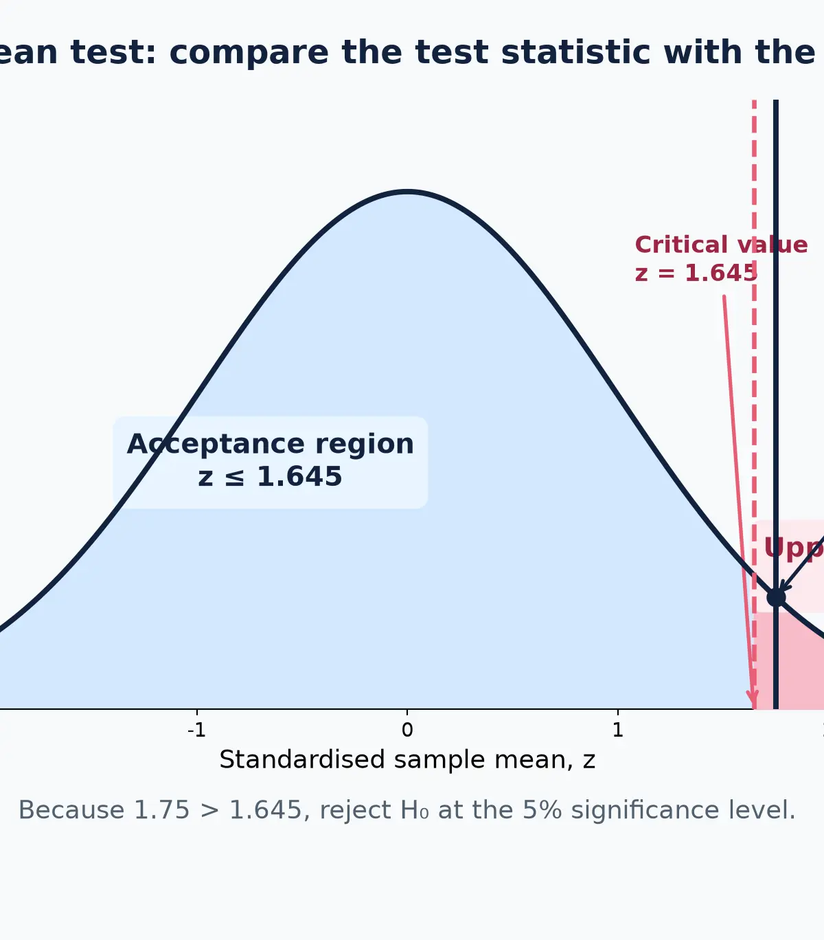
Examiner alert: candidates frequently use σ² as though it were σ. If the question gives a variance, take the square root before calculating the standard error. A question that gives a standard deviation needs no square root.
Key concept 4: correlation tests
For this section, AQA may give you a product moment correlation coefficient r and a p-value or critical value. Do not calculate r unless a separate question asks for it. Write H₀: ρ = 0, which states that there is no linear population correlation. Then choose H₁ to match the wording: ρ > 0, ρ < 0 or ρ ≠ 0.
If a p-value is supplied, compare it directly with α. If a critical value is supplied, compare r, or |r| for a two-tail test, with that value. Your conclusion must use linear correlation. It must not claim that one variable causes the other. A significant correlation can be influenced by a third variable, a non-linear relationship, or the sample design.
Formulae and calculator discipline
| Relationship | Status | When it earns marks |
|---|---|---|
| X ∼ B(n, p₀) | Must memorise / construct from H₀ | State it before a binomial calculation. |
| P(X ≤ c) or P(X ≥ c) | Must memorise | Use the correct cumulative tail to establish a critical region or p-value. |
| x̄ ∼ N(μ₀, σ²/n) | Must memorise / derive from the model | State the distribution of the sample mean under H₀. |
| z = (x̄ − μ₀)/(σ/√n) | Must memorise | Standardise a Normal sample mean. AQA expects candidates to use the standard Normal variable without it being supplied. 3 |
| z = 1.645 for a 5% upper tail; z = ±1.960 for a 5% two-tail test | Must know how to obtain | Use Normal tables or calculator inverse Normal functionality. |
For binomial work, write the event in symbols first. P(X ≥ 11) is usually obtained as 1 − P(X ≤ 10), not 1 − P(X ≤ 11). For Normal work, keep extra figures during the calculation and round the final probability or test statistic sensibly. No unit conversion is normally required in this topic, but the original measurement unit belongs in a contextual conclusion about a mean.
Data, graph and question skills
When a question includes a bar chart, probability table or scatter graph, treat the display as evidence for choosing a model, not as a replacement for the test. A bar chart may make a large binomial count look surprising, but the decision is made only after the correct tail probability has been compared with α. On a standard Normal sketch, shade the tail or tails specified by H₁ before you calculate. This simple habit prevents a one-tail critical value being used in a two-tail question.
For correlation, a scatter graph can suggest a positive or negative pattern, but the test uses the supplied coefficient and critical value or p-value. State the parameter as ρ in the hypotheses, even though the statistic supplied is r. The distinction shows that the sample is being used to infer something about the population.
Read every conclusion back against the original claim. If the question asks whether a mean has increased, the final sentence must say “greater than”, not merely “different”. If it asks whether a proportion has changed, a two-tail test is required even if the sample proportion happens to be lower. These wording checks are quick and protect the interpretation marks.
Practical applications and synoptic thinking
Hypothesis tests support decisions in quality control, medical trials, polling, manufacturing and environmental monitoring. The mathematics is the same whether a “success” is a late delivery, a defective component or a voter supporting a proposal. The only change is the definition of success and the direction of H₁.
There is no required practical for this A-Level Mathematics topic. The examinable practical skill is statistical modelling: define a variable, state the assumptions, carry out the probability calculation and interpret the conclusion without overstating it.
Sources
Visual Resources
2 diagrams and illustrations
Interactive Diagrams
2 interactive diagrams to visualise key concepts
Conceptual Flow Outline
The five-step decision sequence that makes every hypothesis-test answer examinable.
Conceptual Flow Outline
Choose the model from the parameter being tested, then use the matching probability or standardisation method.
Worked Examples
3 worked examples — open one to explore the question and available guidance.
Practice Questions
Try the question, then reveal an answer plan or example response
A café claims that 30% of customers buy a pastry. In 20 independently selected purchases, 3 include a pastry. Test at the 5% level whether the true proportion is lower than 0.30.
Hint: The word “lower” tells you the tail. Start by defining X and writing its distribution under H₀.
A manufacturer claims that 15% of its light bulbs are defective. In a sample of 40 bulbs, 11 are defective. A 5% upper-tail critical region is X ≥ 10. State the hypotheses and test the claim that the defect rate is higher than 15%.
Hint: The critical region has already been supplied. Your job is to compare the observed count with it and interpret.
A medicine bottle is designed to contain a mean of 250 ml. Contents are Normally distributed with known standard deviation 8 ml. A sample of 64 bottles has mean 252 ml. Test at the 5% level whether the mean content differs from 250 ml.
Hint: “Differs” means two-tailed. First calculate the standard error.
For 15 paired observations, r = −0.61. A 1% lower-tail critical value is −0.605. Test whether there is negative linear correlation in the population.
Hint: Use ρ in the hypotheses and remember that more negative values lie further into the lower tail.
A website claims that 60% of visitors complete a form. In a sample of 50 visitors, 23 complete it. Test at the 5% level whether the completion proportion has changed. Explain why a two-tailed binomial critical region may have a total probability below 0.05.
Hint: “Has changed” means two-tailed. Use 0.025 in each tail and choose whole-number boundaries.
Exam technique
How to turn what you know into marks
How to approach the question
Underline the claim and the direction word first. Write H₀ and H₁ before opening the calculator. State the model under H₀, choose the correct tail, then show either a critical-region calculation or a p-value comparison. Finish with a conclusion that names the population parameter and the context.
How to structure your answer
For 3 marks: hypotheses, comparison, contextual conclusion. For 4–5 marks: add definition of X or the distribution under H₀ and a probability calculation. For 6 marks: also show the Normal sample-mean model or full standardisation, and state the significance level in the conclusion.
Timing
Use approximately 1 minute per mark. In the 2-hour, 100-mark AQA Paper 3, a 4-mark hypothesis test should take about 4 minutes, while a 6-mark test should take about 6 minutes.
Common pitfalls
- Writing “accept H₀”. Avoid this by using “do not reject H₀” and “insufficient evidence to conclude…” when the result is not significant.
- Choosing the tail from the observed sample rather than H₁. Avoid this by translating “greater”, “less” and “different” before calculating.
- Using P(X ≤ x) as an upper-tail p-value. Avoid this by writing the event first, then using P(X ≥ x) = 1 − P(X ≤ x − 1).
- Using a Normal mean test where the population variance is unknown. Avoid this by checking the question explicitly gives, knows or assumes the variance.
- Claiming correlation proves causation. Avoid this by concluding only “evidence of linear correlation”.
What the command words want
- Compare
- State both quantities and the inequality, for example “1.75 > 1.645” or “0.029 < 0.05”.
- Explain
- Link the probability boundary to the decision: “Because p < 0.05, the sample is sufficiently unusual under H₀, so reject H₀.”
- Describe
- Identify the region or direction using correct statistical terminology, for example “upper critical region” or “two-tailed test”.
- Evaluate
- State the decision, evidence strength and contextual limitation. For correlation, distinguish association from causation.
- Calculate
- Show the model first, then the calculator event or standardisation. Retain enough figures to support the comparison.
- State/Give
- Write the exact hypothesis, distribution or critical value requested. Keep notation precise: use p, μ or ρ as appropriate.
Watch or listen (optional)
Test your understanding of O: Statistical hypothesis testing
Active recall beats re-reading. Take an instant quiz now to test what you’ve learned and lock it into long-term memory.
7 days Premium · Then the free plan continues · No card, no charge