Select an appropriate probability distribution for a context, with appropriate reasoning, including recognising when the binomial or Normal model may not be appropriate

Overview

Specification reference: Pearson Edexcel A Level Mathematics 9MA0, 4.3. This is a decision-making topic, not a formula-hunting topic. In a Paper 3 context, candidates are given a situation and must decide whether a Binomial, Normal, or no model is justified. The highest-value phrase is not simply “use a Binomial distribution”. It is “a Binomial model is suitable because ...”, followed by the assumptions that the context really meets.

Pearson expects you to select an appropriate probability distribution and recognise when the Binomial or Normal model is inappropriate. That means you must identify the type of variable first. Counts, such as the number of defective bulbs in 40 inspected bulbs, are discrete. Measurements, such as packet mass, time, or height, are continuous. A count may fit a Binomial model only when four conditions hold. A continuous measurement may fit a Normal model only when the distribution is plausibly symmetric and bell-shaped in context. Do not force a model onto data just because a question mentions probability.

On Paper 3, this material connects probability, data presentation, statistical sampling and hypothesis testing. Typical question styles ask you to state a model with parameters, justify it using the context, identify a broken assumption, decide whether a Normal approximation is sensible, or use continuity correction. Paper 3 is 2 hours for 100 marks, so use approximately 1.2 minutes per mark. A 3-mark “state and justify” item should normally take no more than four minutes.

Key Concepts

Concept 1: Start with the random variable

Define what is being counted or measured before selecting a model. Write a sentence such as: “Let (X) be the number of customers, out of 30 selected customers, who renew their subscription.” That wording makes (X) a count, so its possible values are 0, 1, 2, ..., 30. This is a discrete random variable. By contrast, “Let (T) be the time in minutes taken by a customer to complete checkout” is continuous, because any value in an interval is possible.

The model must describe the variable, not merely the setting. “Customers” does not automatically mean Binomial. Counting customers who renew could be Binomial. Measuring their waiting times could be Normal. Recording their preferred payment method is neither a continuous measurement nor necessarily a two-outcome experiment.

Examiner test: ask “Can the answer be 4.7?” If no, the variable is likely discrete. Ask “Is the variable a measured quantity which could take any value in a range?” If yes, Normal may be a possibility.

Figure 1. A Binomial model allocates probability to separate integer counts. A Normal model is continuous, so probability is an area under a smooth curve.

Concept 2: The Binomial model, (X \sim B(n,p))

A Binomial distribution models the number of successes in a fixed number of trials. The word “success” is just the category you choose to count. It could mean a bulb is defective, a student passes, or a customer clicks an advert. Success does not mean desirable.

Before using (X \sim B(n,p)), test all four conditions:

1. Fixed number of trials: there are exactly (n) opportunities.
2. Binary outcome: each trial is classified as success or failure, with no third category.
3. Independent trials: one result does not alter another result’s chance.
4. Constant probability: the success probability is the same (p) on every trial.

For example, a factory independently checks 25 components from a vast production run, with each component having a 0.04 probability of being defective. If (X) is the number defective, (X \sim B(25,0.04)) is reasonable. The number is fixed, each component is defective or not defective, the checks are independent, and (p) is treated as constant.

A common trap is sampling without replacement from a small population. Suppose eight cards are drawn without replacement from a pack containing winners and non-winners. Once a winner is drawn, fewer winners remain, so both independence and constant (p) fail. A Binomial model is not exact. In a 3-mark explanation, candidates should name the broken assumption and connect it to the context: “The draws are not independent because the card is not replaced, so the probability of a winning card changes after each draw.”

Concept 3: The Normal model, (X \sim N(\mu,\sigma^2))

The Normal distribution is a continuous, symmetric, bell-shaped model. It is described by a mean (\mu), which sets the centre, and a variance (\sigma^2), which sets the spread. The standard deviation is (\sigma), not (\sigma^2). Pearson uses the notation (N(\mu,\sigma^2)), while many calculators ask for (\sigma). Write the square root before typing anything into Normal CD.

A Normal model is plausible when the variable is a continuous measurement and the population is reasonably symmetric and unimodal, with no severe outliers or hard boundary causing pronounced skew. Human heights within a sufficiently homogeneous group often provide a plausible model. The times taken to finish a race may not: times cannot be negative and may have a long right tail. The number of sixes in 20 dice throws is not Normal as the original model because it is a discrete count. That count could, under suitable conditions, be approximated by a Normal distribution, but that is a separate claim.

For a continuous variable, (P(X=a)=0). Therefore (P(X<a)=P(X\leq a)). This is unlike a discrete Binomial variable, where (P(X<6)=P(X\leq5)). Credit is given for recognising this difference when translating words into probability notation.

Concept 4: When a Normal approximation to Binomial is justified

Pearson states that (B(n,p)) may be approximated by (N(np,np(1-p))) when (n) is large and (p) is close to 0.5. State both points in a justification. A useful numerical check is that both (np) and (n(1-p)) should be comfortably above 5. This helps identify a distribution that is not too skewed, but the course wording to use is still “(n) is large and (p) is close to 0.5”.

If (p) is near 0 or 1, a Binomial distribution is skewed. For example, (B(80,0.03)) has (np=2.4), so a symmetric Normal curve would be a poor match. Do not write “(n) is large, therefore use Normal” without checking (p). The approximation also fails as a starting point if the original Binomial conditions fail.

When the approximation is appropriate, set (Y\sim N(np,np(1-p))). The mean and variance come from the Binomial distribution. The final essential step is acontinuity correction, because a discrete count is being replaced by a continuous curve.

Figure 2. Use the context to test the model before calculating.

Concept 5: Continuity correction

Each integer value of a Binomial count represents a bar of width 1 on a graph. A Normal curve has no gaps, so move each boundary by half a unit to capture the same region. For (Y), the Normal approximation to (X):

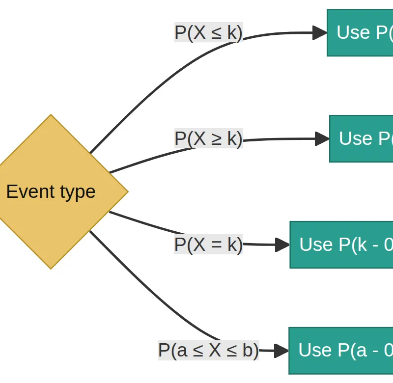
• (P(X\leq k)) becomes (P(Y<k+0.5)).
• (P(X\geq k)) becomes (P(Y>k-0.5)).
• (P(X=k)) becomes (P(k-0.5<Y<k+0.5)).
• (P(a\leq X\leq b)) becomes (P(a-0.5<Y<b+0.5)).

Do not apply a continuity correction to a variable that was originally Normal. It is only used when you are approximating a discrete distribution with a continuous one. A quick sketch of bars centred on the integers prevents the most common sign error.

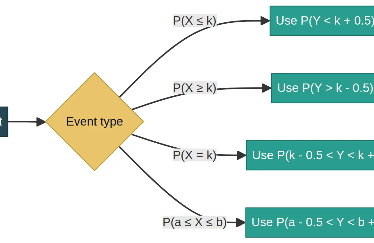
Figure 3. Translate the exact discrete event before using Normal CD.

Mathematical Relationships

Binomial probability:(P(X=x)=\binom{n}{x}p^x(1-p)^{n-x}), where (n) is the number of trials, (x) is the number of successes, and (p) is the probability of success.Given on the Pearson formulae booklet. In practice, calculator Binomial PD and Binomial CD are expected, but write the probability statement first so method marks remain visible.

Binomial mean and variance:(E(X)=np) and (\operatorname{Var}(X)=np(1-p)).Given on the Pearson formulae booklet. These establish the parameters for a Normal approximation.

Normal notation: (X\sim N(\mu,\sigma^2)). Here (\mu) is the mean and (\sigma=\sqrt{\sigma^2}) is the standard deviation. Notation and the Normal distribution form are provided in the Pearson booklet; the interpretation must be understood.

Standardisation: (Z=\dfrac{X-\mu}{\sigma}). Must be understood and used, even if a calculator handles the arithmetic. It explains why a raw observation is compared to the mean in units of standard deviation.

Normal approximation:if suitable, (X\sim B(n,p)) is approximated by (Y\sim N(np,np(1-p))).Must be understood, including the conditions and continuity correction.

Practical Applications and Modelling Judgement

Quality control often creates Binomial contexts. Count the number of defective items in a fixed random sample, then check whether each item can be treated as independent with a stable defect probability. Large, well-mixed production runs make that assumption more credible than a short batch from one faulty machine.

Normal models occur in measurement contexts, including component lengths, packet masses, heights, and instrument error. The practical question is not “does the graph look like a perfect bell?” No real sample does. Ask whether a symmetric, single-peaked approximation is sensible for the decision being made. Strong skew, two distinct groups, an obvious ceiling or floor, or extreme outliers are reasons to challenge the model.

In every model-selection answer, make your assumption visible. The mark is often earned by the phrase after “because”. A candidate who gives correct parameters but no contextual reason risks losing the justification mark. A candidate who identifies a broken assumption and explains its effect has shown the critical modelling judgement required by 4.3.

Calculator discipline

For Binomial CD, write the event in cumulative form first. “At least 6” means (P(X\geq6)=1-P(X\leq5)). For a Normal calculation, write (\sigma=\sqrt{\sigma^2}) and show the continuity-corrected boundary if relevant. Record at least four decimal places from the calculator before giving a final answer, usually to three significant figures unless the question says otherwise.

Audio revision podcast

Use this 10-minute tutor-led recap before a Paper 3 practice session, then complete the quick-fire recall questions without looking at the guide.

Sources used

The authoritative curriculum statements, Paper 3 timing and formulae-booklet guidance are from Pearson Edexcel’s A Level Mathematics Specification, Issue 4 and Mathematical Formulae and Statistical Tables. See the sources field for direct links.