Pearson Edexcel · A-Level · Mathematics
Course version: 9MA0 · Version from Mar 2026
Understand and use simple, discrete probability distributions (calculation of mean and variance of discrete random variables is excluded), including the binomial distribution, as a model; calculate probabilities using the binomial distribution
This guide turns Edexcel Topic 4.1 into a dependable exam routine: define the count, test the binomial assumptions, translate the probability wording, then calculate. It matters because Paper 3 rewards both accurate calculator work and the mathematical judgement needed to model or criticise a real situation.
- 10 min read
- 3 worked examples
- 5 practice questions
- 8 key terms
Check what you remember
Read the wording for your board, then hide it and explain Random variable in your own words. Rough notes are fine. This is a self-check, with no mark or grade.
Reference: Pearson Edexcel
A numerical variable whose value is determined by the outcome of a random experiment.
Study Notes

Overview
Pearson Edexcel A-Level Mathematics Topic 4.1: Statistical Distributions asks candidates to work with simple discrete probability distributions and use the binomial distribution as a real-world model. In a typical question, marks are awarded for communicating a model correctly as well as obtaining a decimal. A calculator is allowed in Paper 3, but it cannot decide whether a model is sensible or translate “at least” accurately for you.
The central idea is that a random variable turns chance into a number. Once a context has been represented by a variable, a distribution describes how likely each possible value is. The binomial distribution is a particularly useful model because it counts the number of successes in a fixed set of similar trials. This links directly to earlier probability work, including complements, independence and conditional probability, and later work on normal approximation and hypothesis tests. Pearson places this content in the statistics section of Paper 3, a two-hour, 100-mark paper. There is no fixed mark allocation for Topic 4.1, so candidates should be ready for quick calculations, model selection and critical comments in context. 1
Examiner rule: define what is being counted before you state a distribution. “Let (X) be the number of…” makes the mathematics unambiguous.
10-minute tutor podcast
Listen once for the model sequence, then pause before each recall prompt and answer aloud. The script mirrors the notation and examiner language used in this guide.
Key Concepts
1. Discrete random variables and probability distributions
A discrete random variable has values that can be listed, normally as whole-number counts. For example, if (X) is the number of defects in five components, then (X) can be (0,1,2,3,4,5). It cannot be 2.7 because we are counting components. This differs from a continuous variable such as mass or time, which may take any value in an interval.
A discrete probability distribution lists each permitted value and its probability. Two non-negotiable checks apply:
[
0 \leq P(X=x) \leq 1 \qquad \text{and} \qquad \sum P(X=x)=1.
]
The second relationship is often tested by giving a table containing (k). Add the probabilities, equate the total to one, and solve. Do not try to find the mean or variance of an arbitrary probability table for this specification point: Pearson explicitly excludes that calculation in Topic 4.1. 1
A discrete uniform distribution is a special case where every listed outcome is equally likely. A fair die gives each face probability (1/6). Uniform does not mean binomial. A die result has six possible outcomes. However, “rolling a six” versus “not rolling a six” has two outcomes, so repeated die rolls can form a binomial experiment.
A fast table workflow
When a question gives a probability table, work in three passes. First, check the support: are all possible values of (X) listed, and are they sensible for the context? A count of late buses cannot be negative or fractional. Second, check the total: add the probability row. If the total is not one, either the table is incomplete or an unknown value must be found. Third, use only the values named in the event. For example, if (P(X=0)=0.2), (P(X=1)=0.5) and (P(X=2)=0.3), then (P(X<2)=P(X=0)+P(X=1)=0.7). Do not add (P(X=2)), because “less than 2” excludes 2.
This short routine is also a defence against calculator overuse. A discrete table is already a complete probability model. Candidates gain credit by showing the relevant addition and by making clear which values are included. Where an event is written in words, convert it to an inequality first, then select the matching rows.
2. The binomial model
Write a binomial model as
[
X \sim B(n,p).
]
Here, (X) is the number of successes, (n) is the fixed number of trials, and (p) is the probability of the defined success on one trial. A “success” is merely the outcome being counted. If a question asks for the number of faulty items, then a fault is the success for that model.
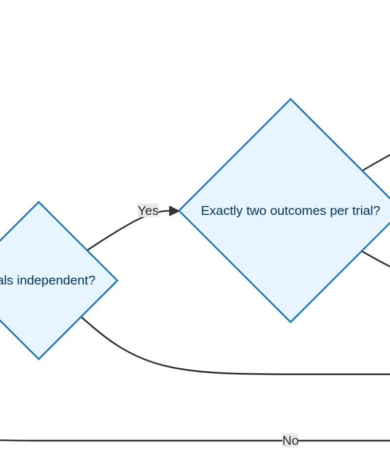
Before using (B(n,p)), test FICT:
- Fixed number of trials: (n) is known before the experiment begins.
- Independent trials: one result does not affect the next.
- Constant probability: (p) stays the same on every trial.
- Two outcomes: each trial is success or failure, relative to the definition of success.
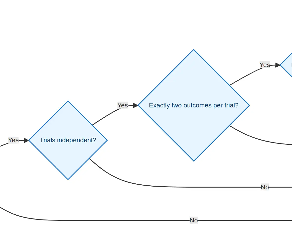
This is more than a checklist to memorise. It explains why a model works. For example, sampling 10 bulbs from a very large production run may be treated as independent, since removing one bulb barely changes the chance that the next is faulty. Sampling 10 sweets without replacement from a small bag is different: each choice changes the composition of the bag, so independence and constant (p) fail.
3. State the model, then translate the words
Suppose 12% of a large population have a stated characteristic and a random sample of 25 is taken. A clear answer is:
[
\text{Let }X\text{ be the number in the sample with the characteristic.}\qquad X\sim B(25,0.12).
]
That model line can earn a mark. It tells the examiner what is counted, the number of trials and the probability of success. It also makes later notation meaningful.
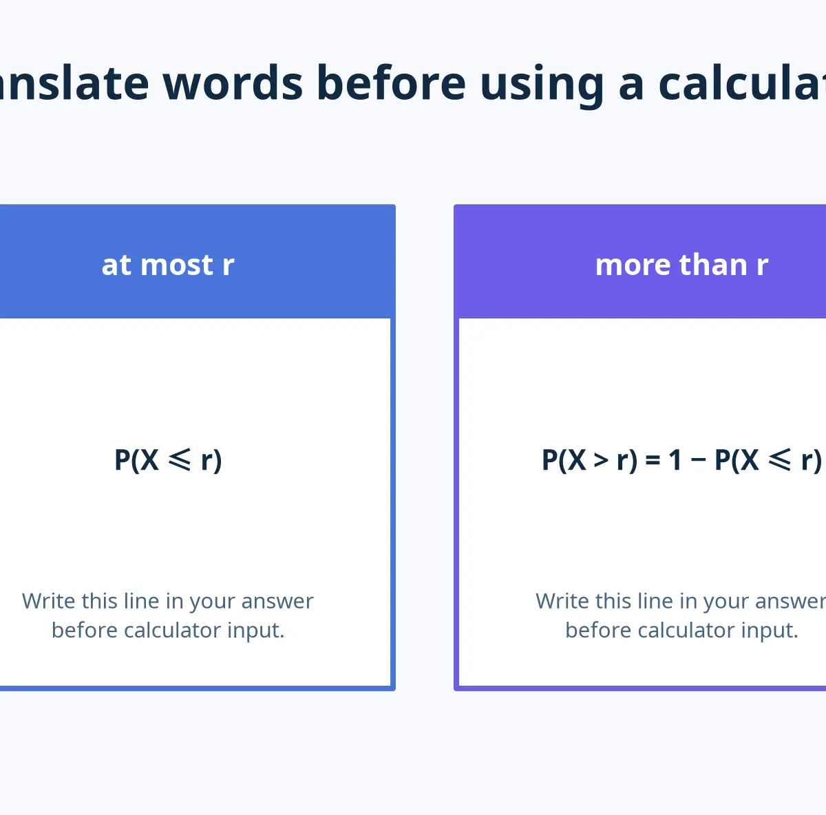
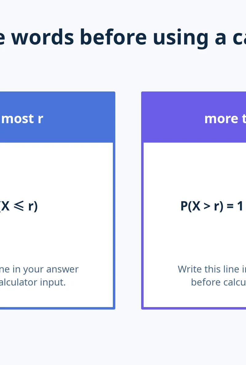
The biggest avoidable error is mistranslating a phrase. Read the boundary word slowly. At most 4 includes 4, so it means (P(X\leq4)). Fewer than 4 excludes 4, so it means (P(X\leq3)). At least 4 includes 4, so it means (P(X\geq4)). More than 4 excludes 4, so it means (P(X>4)).
For an exact probability, use the probability mass function:
[
P(X=r)={n \choose r}p^r(1-p)^{n-r},\qquad r=0,1,\ldots,n.
]
This formula is supplied in the Pearson Edexcel Mathematical Formulae and Statistical Tables booklet. The booklet also provides cumulative binomial tables, but Topic 4.1 expects candidates to use a calculator for individual or cumulative binomial probabilities. 2
4. Calculator method and complements
$Calculator terminology varies, so the mark-winning method is the notation you write before pressing buttons. Use an individual binomial probability function, often called binompdf, for (P(X=r)). Use a cumulative function, often called binomcdf, for (P(X\leq r)). Enter the correct (n), (p) and boundary value, then retain full calculator accuracy until the final answer.$
For right-hand tails, a complement is usually quickest:
[
P(X>r)=1-P(X\leq r),\qquad P(X\geq r)=1-P(X\leq r-1).
]
The (r-1) is crucial. For “at least 3”, the complement is “at most 2”. Candidates lose marks by writing (1-P(X\leq3)), which calculates more than 3 instead.
A full calculation layout looks like this:
[
X\sim B(15,0.08)\
P(X\geq3)=1-P(X\leq2)=0.113\text{(3 s.f.)}.
]
The stated distribution, correct inequality, complement and numerical answer each make the method visible. Credit can therefore be given for a correct approach even if a later calculator entry is mistyped.
5. Shape and reasonableness
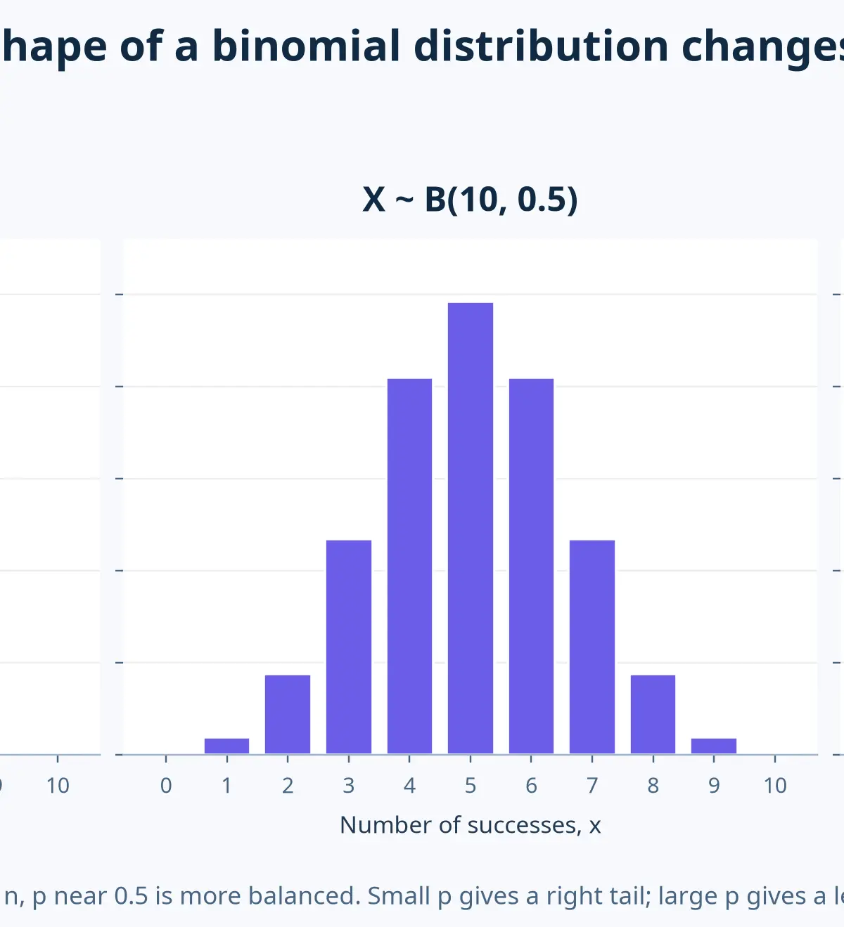
A binomial distribution is discrete, so its graph has separate bars rather than a smooth curve. With (n) fixed, the value of (p) controls the shape. When (p) is close to 0, small counts are most likely and there is a tail to the right. When (p) is close to 1, the tail is to the left. When (p=0.5), the distribution is symmetrical. Use this as a sense check. A very high probability of 10 successes when (p=0.1) should look suspicious.
6. Modelling and critical comments
Pearson expects candidates to model real situations and comment critically on appropriateness. 1 Do not write only “the model may be inaccurate”. Identify the assumption and the consequence. For example:
“The people may not be independent because members of the same household can share the same exposure. This could make the probability of success vary between selections.”
Other strong criticisms include a non-random sample, a changing probability caused by fatigue or depletion, or a trial with more than two relevant outcomes. Conversely, if the sample is random and the population is much larger than the sample, explain why independence is a reasonable approximation.
Mathematical Relationships and Formula Status
| Relationship | Use | Formula-booklet status |
|---|---|---|
| (\sum P(X=x)=1) | Find a missing probability or check a distribution | Must memorise and understand |
| (0\leq P(X=x)\leq1) | Check validity | Must memorise and understand |
| (X\sim B(n,p)) | State a binomial model | Must memorise notation and meaning |
| (P(X=r)={n\choose r}p^r(1-p)^{n-r}) | Exact binomial probability | Given on formula sheet 2 |
| (P(X>r)=1-P(X\leq r)) | “More than” tail | Must memorise and understand |
| (P(X\geq r)=1-P(X\leq r-1)) | “At least” tail | Must memorise and understand |
Practical Applications
Binomial models appear whenever the same yes-or-no criterion is repeated: the number of packages arriving damaged, the number of customers replying to an email, or the number of components passing a test. In each case, you must decide whether the four FICT conditions are credible. This is why the topic is more than calculator work. A quality-control question may have a perfect numerical answer but still require a warning that items from the same batch could be correlated.
Exam Technique
Paper 3 has 100 marks in 120 minutes, so budget about 1.2 minutes per mark. For a 3-mark binomial calculation, write the model and probability statement swiftly, calculate, and round only at the end. For a 5- or 6-mark modelling question, spend more time on context-linked reasoning. Use the command word as a guide: state needs the concise notation; calculate needs working; explain needs the condition and why it holds or fails; comment or critique needs a realistic limitation.
References
Visual Resources
2 diagrams and illustrations
Interactive Diagrams
2 interactive diagrams to visualise key concepts
Conceptual Flow Outline
A decision path for establishing a valid binomial model using FICT.
Conceptual Flow Outline
Translate common probability phrases before selecting a calculator function.
Worked Examples
3 worked examples — open one to explore the question and available guidance.
Practice Questions
Try the question, then reveal an answer plan or example response
The values of X are 0, 1 and 2. Their probabilities are 0.10, k and 0.35 respectively. Find k.
Hint: A complete probability distribution has total probability 1.
A component fails with probability 0.10. Twelve components are tested independently. Let X be the number that fail. State the distribution of X and find P(X = 0).
Hint: The event X = 0 means no components fail.
For X ~ B(10, 0.30), calculate the probability of exactly 3 successes.
Hint: ‘Exactly’ is an equality, not a cumulative probability.
For X ~ B(20, 0.15), calculate the probability of more than 4 successes.
Hint: The complement of ‘more than 4’ is ‘at most 4’.
A bag contains 3 red counters and 9 blue counters. Seven counters are drawn without replacement. Let X be the number of red counters drawn. A student claims that X ~ B(7, 0.25). Evaluate this claim.
Hint: Test every part of FICT, not just the initial value of p.
Exam technique
How to turn what you know into marks
How to approach the question
Underline the quantity being counted and define X. Run FICT before claiming binomial. Translate the wording into P(X = r), P(X ≤ r), P(X > r) or P(X ≥ r) before using the calculator. For a criticism, identify the failed assumption and connect it to the context.
How to structure your answer
For 1–2 marks, write the model or probability statement precisely. For 3–4 marks, show model → notation → calculator value. For 5–6 marks, add a context-specific justification or critique, with one developed point per requested assumption.
Timing
Paper 3 is 120 minutes for 100 marks, so allow about 1.2 minutes per mark overall. A 6-mark modelling question should normally receive about 7 minutes, including a quick reasonableness check.
Common pitfalls
- Writing P(X ≤ r) for ‘fewer than r’. It should be P(X ≤ r − 1), because r itself is excluded.
- Using 1 − P(X ≤ r) for ‘at least r’. This gives more than r; use 1 − P(X ≤ r − 1).
- Stating a binomial model when sampling without replacement from a small population. Explain that independence and constant p can fail.
- Rounding a cumulative probability before taking a complement. Keep full calculator precision until the final line.
What the command words want
- Compare
- Identify what changes between the two contexts, especially n, p, independence or the distribution shape.
- Explain
- Name the binomial condition and use ‘because’ to tie it to the scenario.
- Describe
- Say what the probability phrase includes or excludes, using an inequality where helpful.
- Evaluate
- Consider whether the assumptions are realistic, give a specific limitation and reach a justified conclusion about the model.
- Calculate
- Show the model and probability notation before the calculator result; round only at the end.
- State/Give
- Give a concise mathematical statement, for example X ~ B(20, 0.15). Do not add irrelevant calculation.
Watch or listen (optional)
Test your understanding of Understand and use simple, discrete probability distributions (calculation of mean and variance of discrete random variables is excluded), including the binomial distribution, as a model; calculate probabilities using the binomial distribution
Active recall beats re-reading. Take an instant quiz now to test what you’ve learned and lock it into long-term memory.
7 days Premium · Then the free plan continues · No card, no charge