Understand and use the Normal distribution as a model; find probabilities using the Normal distribution; link to histograms, mean, standard deviation, points of inflection and the binomial distribution

Overview

Normal distribution questions reward disciplined interpretation rather than obscure mathematics. In Pearson Edexcel A-Level Mathematics 9MA0, specification point 4.2 requires candidates to use the Normal distribution as a model, calculate probabilities, connect the model with histograms, mean, standard deviation and inflection points, and approximate a binomial distribution where appropriate. You will usually meet this on Paper 3, but Pure Mathematics is assumed knowledge on that paper, so algebra and graph interpretation can appear inside a statistics context.

A strong answer makes the distribution, event and method visible. Candidates must read X ∼ N(μ, σ²) accurately, decide whether the required area is left, right or between two values, and enter the standard deviation, not the variance, into the calculator. The most demanding questions ask for an unknown parameter using inverse Normal or simultaneous equations, or combine binomial modelling with a continuity correction. The good news is that each question follows a repeatable routine: model, sketch, boundaries, calculator, statement.

Key Concepts

1. Reading the model: centre and spread

The notation X ∼ N(μ, σ²) says that the continuous random variable X is modelled by a Normal distribution. The first parameter, μ, is the mean. It places the centre of the curve. The second parameter is the variance, σ², not the standard deviation. Therefore, when a calculator asks for a standard deviation, use σ = √(σ²).

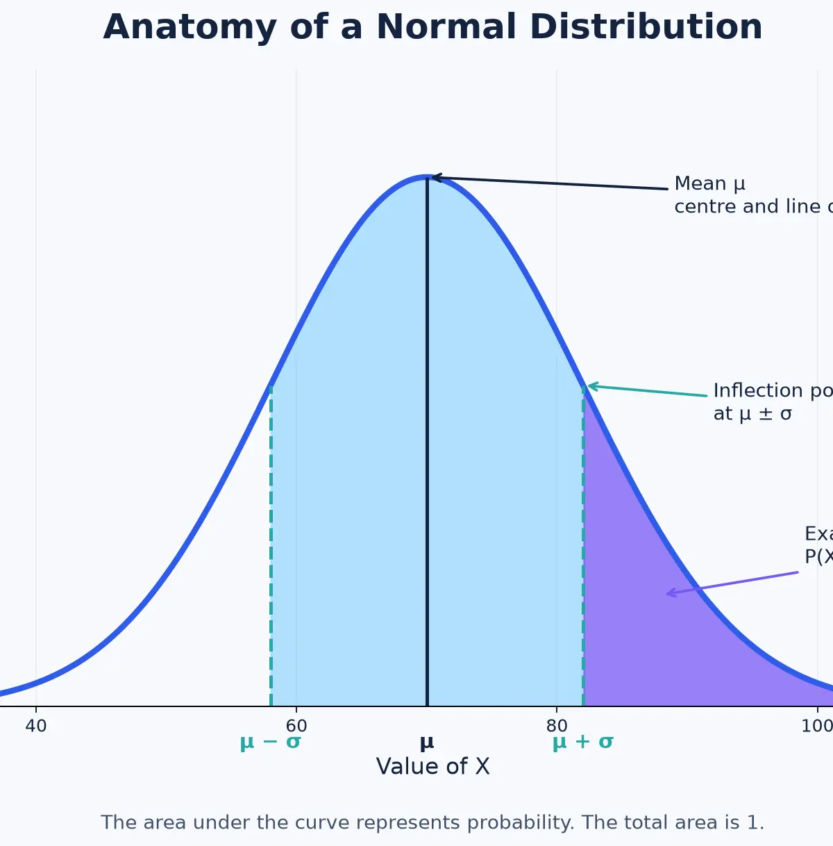
The curve is bell-shaped and symmetric about x = μ. Moving μ shifts the whole curve left or right. Increasing σ spreads the values further from the mean, so the curve becomes wider and lower while retaining total area 1. The area under a continuous curve is probability, so P(X = a) = 0: a single exact value has no area. Only intervals carry probability.

Example: If X ∼ N(70, 144), then μ = 70, Var(X) = 144 and σ = 12. The centre is 70, not 144. A candidate who inputs 144 as the standard deviation creates a wildly over-spread model and loses accuracy marks.

2. Shape, histograms and inflection points

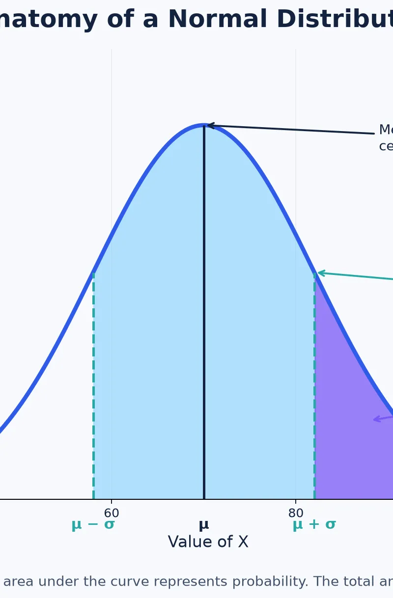
For a Normal model, the curve is unimodal and symmetric. The two points of inflection are at x = μ − σ and x = μ + σ. They are the points at which the curve changes concavity. Pearson Edexcel requires candidates to know this result, but not to derive it. For X ∼ N(70, 144), the inflection points are 70 − 12 = 58 and 70 + 12 = 82.

Link the model to a histogram carefully. In a histogram, area represents frequency, not height alone. A continuous, roughly symmetric, single-peaked histogram with no major outliers may be reasonably modelled by a Normal curve. A strong evaluation answers in context: “The model may be unsuitable because the histogram is positively skewed, so it is not symmetric about a central mean.” Do not merely write “it does not look normal”. A bimodal pattern, a marked skew, a ceiling effect or influential outliers all weaken the model.

3. Probabilities: translate words into an area

Before touching the calculator, translate the event.

• P(X < a) is the left-hand area up to a.
• P(X > a) is the right-hand tail beyond a.
• P(a < X < b) is the area between a and b.

On a calculator, Normal cumulative distribution is usually entered with a lower bound, upper bound, mean and standard deviation. For an upper tail, use a as the lower bound and a very large number as the upper bound. For a lower tail, use a very negative lower bound and a as the upper bound. For a middle interval, enter both stated limits. Sketching the region first prevents the classic “wrong tail” error.

Example: For X ∼ N(70, 144), P(X > 85) is the shaded right tail beyond 85. Since σ = 12, P(X > 85) = P(Z > (85 − 70)/12) = P(Z > 1.25) = 0.10565…, so P(X > 85) = 0.106 to three significant figures.

4. Standardisation and inverse Normal

Standardisation rescales a Normal variable so that it can be compared with the standard Normal distribution: Z ∼ N(0, 1). Use

Z = (X − μ) / σ **[Must memorise and use]**This tells the examiner how many standard deviations a value lies from the mean. Standardisation is essential when using Normal tables and is a transparent way to set up unknown-parameter questions. Keep unrounded calculator values where possible, then round only the final answer.

Inverse Normal reverses a probability calculation. A cumulative probability is known and the boundary is required. If P(X < t) = 0.975, use inverse Normal to find the 97.5th percentile. For X ∼ N(18, 12.25), σ = 3.5 and the z-value is about 1.960. Hence t = 18 + 1.960(3.5) = 24.86…, giving 24.9 to three significant figures. Remember: Normal cumulative gives an area from a value; inverse Normal gives a value from an area.

5. Finding unknown μ and σ

Questions may supply two probabilities and ask candidates to solve simultaneous equations. Convert each stated probability to a standardised z-value, then return to the original scale. Suppose P(X < 58) = 0.2000 and P(X > 74) = 0.1000.

P(X < 58) = 0.2 gives z = −0.8416, so 58 = μ − 0.8416σ.

P(X < 74) = 0.9 gives z = 1.2816, so 74 = μ + 1.2816σ.

Subtracting gives 16 = 2.1232σ, so σ = 7.536…. Substitution gives μ = 64.342…. The algebra is where method marks sit. State both equations before solving. Credit can be given for a correct method even when a candidate’s sensible rounding changes the final decimal.

6. Binomial approximation and continuity correction

Pearson Edexcel requires the link between a binomial model and a Normal approximation. When B ∼ B(n, p), n is large and p is close to 0.5, then

B(n, p) ≈ N(np, np(1 − p)) **[Must memorise]**The approximate Normal mean is np; its variance is np(1 − p). The expectation and variance for a binomial distribution are supplied in the formulae booklet, but candidates must select and apply them. State the condition in the wording above. Pearson guidance makes clear that np > 5 and n(1 − p) > 5 alone do not earn full credit unless n is also described as large.

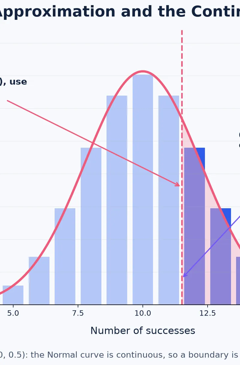
A binomial random variable is discrete, but a Normal distribution is continuous. The continuity correction aligns the continuous area with discrete bars:

• P(B ≥ k) ≈ P(Y > k − 0.5)
• P(B ≤ k) ≈ P(Y < k + 0.5)
• P(B = k) ≈ P(k − 0.5 < Y < k + 0.5)

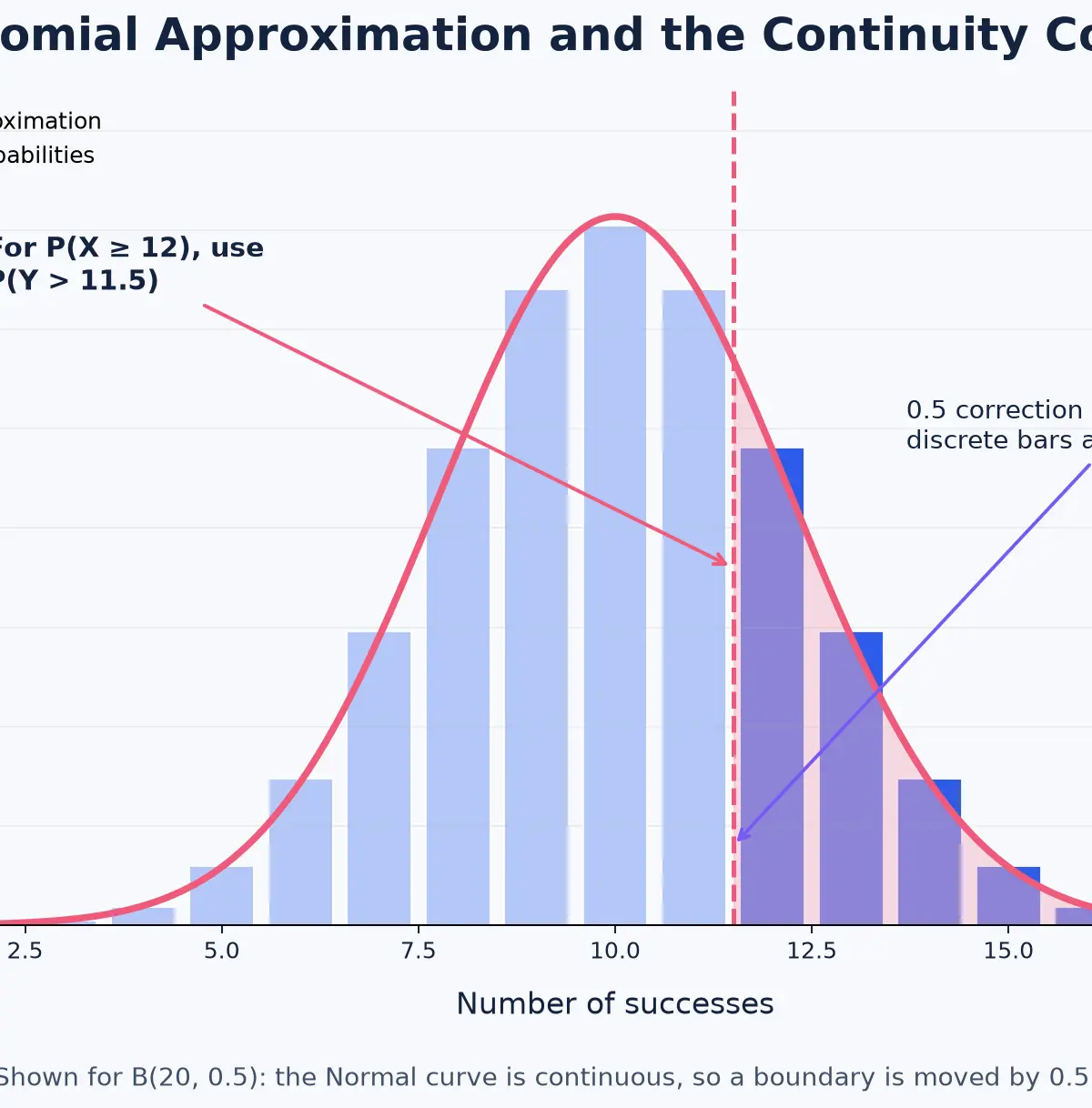
Example: If B ∼ B(80, 0.55), then Y ∼ N(44, 19.8) and σ = √19.8 = 4.45…. To estimate P(B ≥ 50), use P(Y > 49.5), not P(Y > 50). This gives P(Z > (49.5 − 44)/4.45…) = 0.108…, so the estimate is 0.108.

Mathematical Relationships and Formula Status

• X ∼ N(μ, σ²): Given in the formulae/statistical tables, but interpretation must be secure. μ is the mean and σ² is the variance.
• σ = √Var(X): Must use. A calculator asks for σ in its Normal distribution function.
• Z = (X − μ)/σ: Must memorise/use. It standardises values and supports table or algebraic methods.
• Inflection points x = μ ± σ: Must memorise. Derivation is not required.
• B(n,p) ≈ N(np, np(1 − p)): Must memorise/use, with “n is large and p is close to 0.5”.
• Continuity correction of 0.5: Must apply whenever a discrete binomial probability is approximated by the continuous Normal model.

The Pearson Edexcel formulae booklet and statistical tables are provided in assessment. Pearson expects calculator use for Normal probabilities. Percentage-points tables or calculator inverse Normal functions can be used to recover z-values. The probability density function and derivations of the Normal mean, variance and cumulative distribution function are not required for this specification point.

Graph and Data Skills

A Normal curve is a model, not proof that the data are Normal. When a histogram is supplied, inspect symmetry, number of peaks, tails and outliers. Refer to the area of bars when explaining frequency. If class widths differ, height is frequency density, so a bar’s height alone cannot be compared as a frequency. Use the mean as the central line of symmetry, use μ ± σ to locate inflection points, and say whether the visual evidence supports the assumptions of a continuous, symmetric model.

Exam-Ready Applications

Normal models are used for continuous measurements such as manufactured lengths, test scores or package masses, but a credible answer still comments on context. A production process may be approximately Normal when many small independent influences act on measurement, yet the model can fail if the instrument rounds heavily, a minimum or maximum value truncates the data, or two different populations have been mixed. In a modelling question, candidates gain credit for a precise reason linked to the actual graph or situation.

Podcast Revision

Listen once with the guide open, then pause the quick-fire quiz and answer aloud before the tutor reveals each answer.

Specification Source

This guide is aligned to Pearson Edexcel A-Level Mathematics 9MA0, section 4.2, including the official enhanced guidance on standardisation, inverse Normal, modelling suitability and the Normal approximation to B(n,p): https://qualifications.pearson.com/content/dam/pdf/A%20Level/Mathematics/2017/specification-and-sample-assesment/pearson-edexcel-l3-advanced-gce-mathematics-9ma0-enhanced-content-guidance-issue-2.pdf