Pearson Edexcel · A-Level · Mathematics
Course version: 9MA0 · Version from Mar 2026
Use logarithmic graphs to estimate parameters in relationships of the form y = axⁿ and y = kbˣ, given data for x and y
Logarithmic graphs are the examiner’s shortcut from a curved data pattern to a usable model. Master the two transformations and you can turn a line’s gradient and intercept into the parameters of power and exponential relationships, with clear method marks available at every stage.
- 10 min read
- 3 worked examples
- 5 practice questions
- 8 key terms
Check what you remember
Read the wording for your board, then hide it and explain Linearisation in your own words. Rough notes are fine. This is a self-check, with no mark or grade.
Reference: Pearson Edexcel
Transforming a non-linear relationship into a linear relationship so that it can be represented by a straight-line graph.
Study Notes

Pearson Edexcel A-Level Mathematics 6.6: Logarithmic Graphs for Estimating Parameters
Overview
Logarithmic graphs turn awkward curves into straight lines. That matters because a straight line reveals its gradient and intercept, and those two values unlock the unknown constants in a model. In Pearson Edexcel 6.6, candidates are expected to estimate parameters in the power model (y=ax^n) and the exponential model (y=kb^x), using data for (x) and (y). The mathematical skill is not merely pressing log on a calculator: it is choosing the correct transformed variables, matching the result to (Y=mX+c), and converting logarithmic values back to original parameters.
This topic links the logarithm laws in 6.4 to exponential growth and decay modelling in 6.7. Typical questions provide a transformed graph, its line of best fit, or data to transform and plot. They may ask you to show that, plot, estimate, determine or state a model. The decisive distinction is where the variable sits: if it is raised to a power, use a log-log plot; if it is itself in the exponent, use a semi-log plot. Marks are often lost by using the right calculation on the wrong axes.
Key Concepts
1. Linearisation: the reason logarithms are used
A relationship is linear when it can be written as (Y=mX+c). A power or exponential curve is not a straight line on ordinary axes, so its gradient and intercept do not directly give the parameters we need. Taking logarithms rewrites the relationship in a linear form. This process is called linearisation.
The essential logarithm laws are:
- (\log(uv)=\log u+\log v)
- (\log(u^r)=r\log u)
- (\log_r A=c \iff r^c=A)
The base can be 10 or (e), but it must be used consistently. If the graph uses (\log_{10}), undo a logged intercept or gradient with a power of 10. If it uses (\ln), undo it with a power of (e). In all cases, quantities put into a real logarithm must be positive. For a power model this means (x>0) and (y>0); for an exponential model, (y>0).
Examiner focus: Credit is given for a correct linear equation before any parameters are read. Write the equation first. It acts as an audit trail for your axis choice.
2. Power relationships: (y=ax^n)
In (y=ax^n), the variable (x) has the power (n). Take logs of both sides:
[\log y=\log(ax^n)=\log a+\log(x^n)=\log a+n\log x.]
Put (Y=\log y) and (X=\log x). Then
[Y=nX+\log a.]
$This matches (Y=mX+c) exactly. Therefore, plot (\log y) against (\log x). The gradient is (n), and the vertical intercept is (\log a), not (a). With base-10 logs, (a=10^c); with natural logs, (a=e^c).$
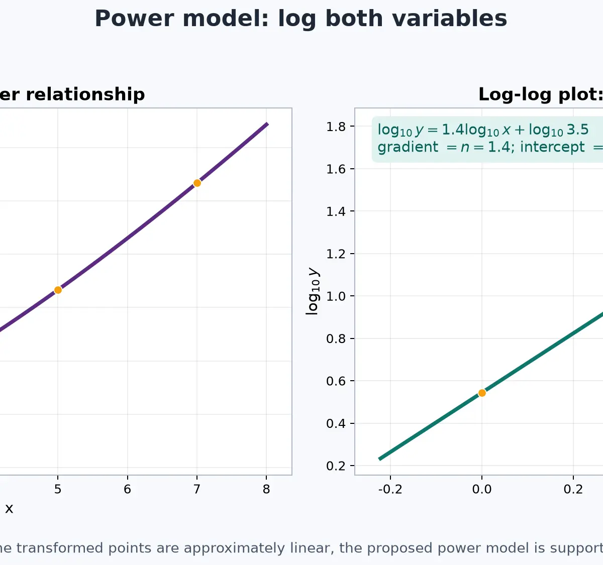
The word against is an axis instruction. “Plot (A) against (B)” means vertical axis (A), horizontal axis (B). Reversing them gives the reciprocal gradient, so it changes the model. Use two widely separated points on the line of best fit, not necessarily two original data points, when calculating a gradient. Graph estimates should be rounded sensibly to the precision the scale supports.
Why this works: logarithms convert multiplication into addition and powers into multipliers. The curved effect of the exponent is therefore absorbed into one constant gradient.
3. Exponential relationships: (y=kb^x)
In (y=kb^x), the variable is in the exponent. The transformation is different:
[\log y=\log(kb^x)=\log k+x\log b.]
This is already in straight-line form if (Y=\log y) and (X=x):
[Y=(\log b)X+\log k.]
$So plot (\log y) against (x). Do not log (x). The gradient is (\log b), while the intercept is (\log k). For base-10 logs:$
[b=10^{\text{gradient}},\qquad k=10^{\text{intercept}}.]
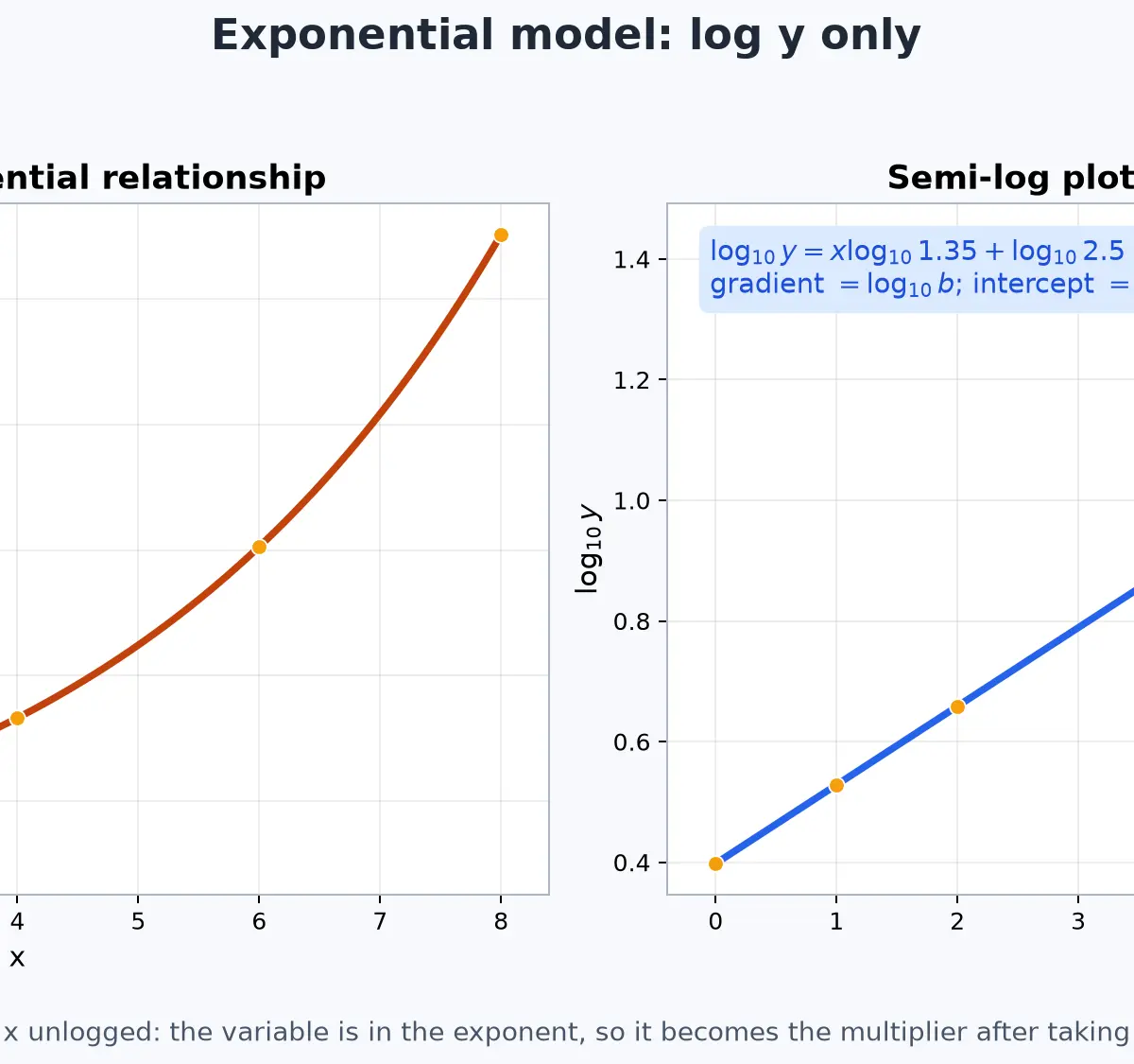
A positive transformed gradient gives (b>1), so the model represents growth. A negative transformed gradient gives (0<b<1), so it represents decay. At (x=0), (y=kb^0=k), so (k) has the useful interpretation of the initial value. Candidates who write “gradient = (b)” have not completed the parameter recovery step and cannot receive the associated marks.
4. Reading and checking a fitted line
A transformed plot that is approximately straight supports the proposed model over the data range. It does not prove that the model is exact, and it does not automatically justify extrapolating far beyond the data. Experimental or rounded data normally sit around, rather than exactly on, a line of best fit.
If the vertical intercept lies off the printed graph, calculate it. Choose a readable point ((X,Y)) on the fitted line and use (Y=mX+c), giving (c=Y-mX). Then apply the relevant antilogarithm. This is often a high-value step because it tests algebra, graph reading and logarithms together.
Accuracy check: substitute a convenient original (x)-value into your final model and see whether it predicts a plausible (y)-value. Also check that a growth factor is greater than 1 and a decay factor is between 0 and 1. These checks do not replace working, but they catch sign and antilog errors.
Mathematical Relationships and Formula Status
All relationships below are must memorise for this topic. They are not a routine formula-sheet substitute.
- Power model: (y=ax^n), where (a>0), (x>0), (y>0). Its linear form is (\log y=n\log x+\log a). Plot (\log y) against (\log x); gradient (=n), intercept (=\log a).
- Exponential model: (y=kb^x), where (k>0), (b>0), (b
eq1), (y>0). Its linear form is (\log y=x\log b+\log k). Plot (\log y) against (x); gradient (=\log b), intercept (=\log k). - Base-10 recovery: if (\log_{10}q=c), then (q=10^c).
- Natural-log recovery: if (\ln q=c), then (q=e^c).
- Line equation: (Y=mX+c), and therefore (c=Y-mX) when an intercept is off-scale.
No unit conversion is intrinsic to this sub-topic. Keep the units carried by (x) and (y) in the final contextual model. Do not take a logarithm of a dimensional value in a formal scientific derivation without a reference unit; in A-Level graph questions, follow the transformed variables specified by the question.
Graph and Data Skills Checklist
- Identify the proposed model before touching the data table.
- Derive the log form, using the same base throughout.
- Make a transformed data table to suitable decimal places.
- Put the word before “against” on the vertical axis.
- Label both transformed axes clearly, including the base if supplied.
- Draw a line of best fit, then take two well-separated points from that line.
- Map gradient and intercept back to the original parameters, using an antilogarithm where required.
- State the final model and interpret it in context.
From a Data Table to a Defensible Model
When a question gives raw data rather than a ready-drawn graph, the transformation table is part of the mathematical argument. For (y=ax^n), add columns headed (\log x) and (\log y). For (y=kb^x), add only (\log y); retain the original (x) column. Copy enough calculator digits into the table to plot accurately, usually three decimal places unless the question indicates otherwise. Do not round each log so aggressively that several points collapse together on the graph.
Choose a scale that uses most of the available graph paper and makes the transformed points spread out. A linear scale is required on each transformed axis. Label a base-10 axis (\log_{10}y), rather than merely “log”, if the question has specified that base. A candidate can have excellent calculations but lose credit for unclear or reversed axes because the graph no longer communicates the required transformation.
After plotting, the line of best fit should pass through the centre of the cloud of points, with a roughly balanced scatter above and below. It does not need to touch every point. Read two convenient coordinates from the line, preferably grid intersections far apart. Then show the subtraction in the gradient calculation. For example, on a log-log plot, (n=(Y_2-Y_1)/(X_2-X_1)). This makes it clear that the gradient belongs to transformed variables, not to the original curve.
A Mark-by-Mark Decision Routine
$For a show that question, begin with the original model and take logs of both sides. Each correct law can earn credit: product law, power law, then a clear rearrangement into (Y=mX+c). Do not jump from (\log(ax^n)) to the final line with no visible reasoning if the question is assessing logarithm laws.$
$For a plot question, the marks normally come from transformed values, sensible scales, correctly labelled axes, accurate plotting and an appropriate line of best fit. Read the precise wording: plotting (\log y) against (x) is not interchangeable with plotting (\log y) against (\log x). It identifies a different family of models.$
For an estimate or determinequestion, a complete answer is a chain: fitted-line gradient (\rightarrow) transformed parameter (\rightarrow) antilogarithm (\rightarrow) original model. If the final answer comes from a graph, use an estimate sign or sensible rounding. If the model represents a real quantity, finish with one sentence about the meaning of the coefficient or multiplier. That last sentence is often where interpretation marks are awarded.
Worked Graph Reading Micro-Example
Suppose the line on a graph of (\log_{10}y) against (x) passes through ((2,0.90)) and ((8,1.62)). The gradient is ((1.62-0.90)/(8-2)=0.12), so (\log_{10}b=0.12) and (b=10^{0.12}\approx1.32). Find the intercept with (c=0.90-0.12(2)=0.66). Thus (\log_{10}k=0.66), so (k=10^{0.66}\approx4.57). The model is (y\approx4.57(1.32)^x). Notice the order: neither 0.12 nor 0.66 appears in the final model because both are logged quantities.
Practical Applications
This is a mathematical modelling skill, not a required practical. In real data, a power model can describe how a quantity changes with scale, such as a biological relationship between mass and metabolic measure. An exponential model can describe repeated percentage change, such as population growth, drug concentration decline or compound interest. The transformed graph lets a scientist or analyst estimate a growth factor or exponent from noisy observations.
The examiner’s judgement is cautious: a straight-ish transformed plot supports a model only across the observed data range. For example, population growth may later slow because resources are limited. A robust answer distinguishes “the fitted model predicts” from “this must happen indefinitely”. This links directly to 6.7, where candidates consider limitations and refinements of exponential models.
10-Minute Audio Revision Podcast
Listen once with the guide open, then listen again with the equations covered. Pause after each recall question and say the linear form aloud before checking it.
Visual Resources
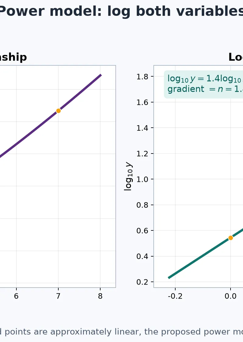
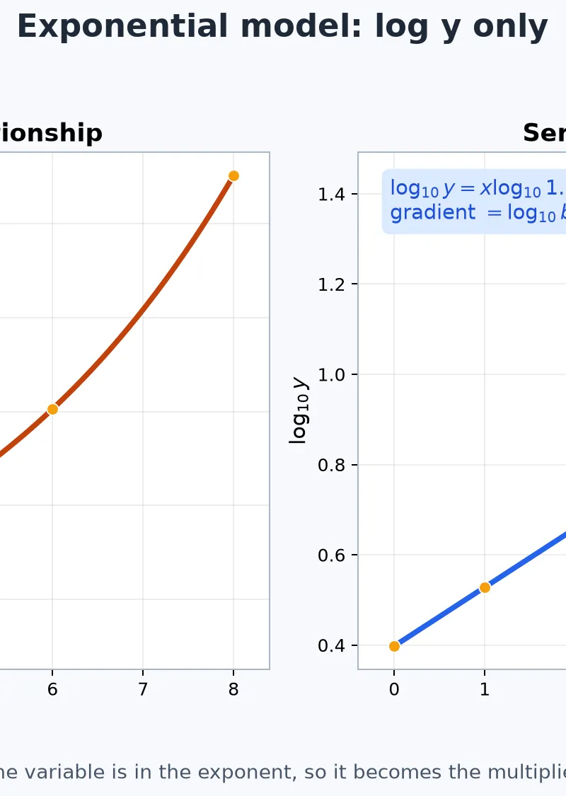
2 diagrams and illustrations
Interactive Diagrams
2 interactive diagrams to visualise key concepts
Conceptual Flow Outline
Decision route for selecting the correct axes and parameters. The position of x determines the transformation.
Conceptual Flow Outline
Parameter-recovery sequence, including the crucial choice of the correct antilogarithm.
Worked Examples
3 worked examples — open one to explore the question and available guidance.
Practice Questions
Try the question, then reveal an answer plan or example response
For (y=7x^{-0.4}), state the variables to plot to obtain a straight line and state the gradient and vertical intercept. [3 marks]
Hint: First take \(\log_{10}\) of both sides and compare with \(Y=mX+c\).
A log-log graph has equation (\log_{10}P=2.1\log_{10}Q-0.3010). Find P in terms of Q. [3 marks]
Hint: Match with \(\log P=n\log Q+\log a\), then remove the base-10 log from the intercept.
For (N=120(0.82)^t), state the axes needed for a straight-line graph of transformed data and explain why its gradient is negative. [4 marks]
Hint: This is an exponential model. The gradient on the transformed graph is \(\log 0.82\).
On a graph of (\ln y$) against x, the line has gradient (-0.35) and passes through ((2,1.10)). The model is (y=ab^x). Determine a and b to 3 significant figures. [5 marks]$
Hint: First find the intercept using \(c=Y-mX\). Then remember that \(c=\ln a\) and \(m=\ln b\).
A student plots (\log_{10}y) against (\log_{10}x) and obtains an approximately straight line with gradient 0.62 and intercept 1.15. Assess whether (y=kb^x) is the most appropriate claimed model, and give the model supported by the graph. [5 marks]
Hint: Use the axes, not the word ‘straight’, to decide the original relationship.
Exam technique
How to turn what you know into marks
How to approach the question
Start by circling the proposed model. Take logs and write its linear form directly beneath it. Label \(Y\), \(X\), \(m\) and \(c\) before reading the graph. For data questions, create the required transformed columns, plot the specified axes, use a line of best fit, then convert every logged parameter back before stating the original model.
How to structure your answer
For 3-4 marks: show the linear form, identify gradient/intercept, recover any logged parameter, then state the model. For 5-6 marks: also show the gradient calculation from well-separated fitted-line points, calculate an off-scale intercept if needed, round sensibly and interpret the model in context.
Timing
Allow approximately 1 minute per mark. A 4-mark parameter question should usually take 4-5 minutes, including a final check; do not spend most of the time plotting if the line equation is already supplied.
Common pitfalls
- Plotting \(\log y\) against \(\log x\) for \(y=kb^x\). Avoid this by deriving \(\log y=x\log b+\log k\): x is already the horizontal variable.
- Treating a vertical intercept as \(a\) or \(k\). Write \(\log a=c\) or \(\log k=c\), then show the antilogarithm.
- Using \(10^c\) to undo \(\ln\). Match the inverse to the log base: \(e^c\) reverses \(\ln\).
- Reading a gradient from two nearby data points. Choose two well-separated points on the drawn line of best fit to reduce graph-reading error.
- Giving excessive precision from a graph. Keep accurate calculator values internally but round the final estimate to the scale or the question’s instruction.
What the command words want
- Plot
- Construct the requested transformed columns, use clear linear scales, place the first named quantity on the vertical axis, and label each axis precisely.
- State
- Give the requested value or model succinctly, but ensure it is the original parameter rather than its logarithm.
- Explain
- Use a cause-and-effect sentence, for example: ‘The gradient is negative, so \(\log b<0\), hence \(0<b<1\), therefore the model shows decay.’
- Estimate
- Use the line of best fit rather than assuming individual data are exact. State parameters to sensible precision and use ≈ where appropriate.
- Show that
- Start from the given model and use logarithm laws one step at a time. End by matching your result to \(Y=mX+c\).
- Determine/Find
- Show coefficient comparison and the antilogarithm. A bare final model may not earn method marks.
Watch or listen (optional)
Test your understanding of Use logarithmic graphs to estimate parameters in relationships of the form y = axⁿ and y = kbˣ, given data for x and y
Active recall beats re-reading. Take an instant quiz now to test what you’ve learned and lock it into long-term memory.
7 days Premium · Then the free plan continues · No card, no charge