Pearson Edexcel · GCSE · Mathematics
Course version: 1MA1 · Version from Mar 2026
Probability: relate relative expected frequencies to theoretical probability, using appropriate language and the 0-1 probability scale
Does a drawing pin have a 50–50 chance just because it can land two ways? Learn to distinguish theoretical probability from experimental estimates, use the 0–1 scale precisely, and write evidence-based answers that earn calculation and explanation marks.
- 14 min read
- 4 worked examples
- 7 practice questions
- 13 key terms
Try the lesson
The start of the Probability: relate relative expected frequencies to theoretical probability, using appropriate language and the 0-1 probability scale lesson, made from checked teaching notes for this specification point.
Have a go first
A fair six-sided dice is rolled 300 times. Work out the expected number of times the dice lands on a 4.
There is more to this lesson
The full lesson goes on to check your understanding and help you earn the marks. Create a free account to carry on, with your progress saved.
7 days Premium · Then the free plan continues · No card, no charge
Check what you remember
Read the wording for your board, then hide it and explain Probability in your own words. Rough notes are fine. This is a self-check, with no mark or grade.
Reference: Pearson Edexcel
A numerical measure of the likelihood of an event, from 0 to 1 inclusive.
Study Notes

Download the complete JSON study guide
Overview
A drawing pin lands point up 37 times in 100 drops. Is its probability 0.37, one half, or something else? This topic teaches you to distinguish a probability calculated from a fair model from an estimate calculated from experimental results. That distinction prevents several common GCSE errors and helps candidates write convincing explanations.
Every probability belongs on the scale from 0 to 1. You will connect fractions, decimals and percentages to words such as impossible, unlikely, even chance, likely and certain. You will calculate relative frequencies, compare them with theoretical probabilities, and explain why larger, well-conducted experiments usually provide more reliable estimates.
For Pearson Edexcel GCSE Mathematics 1MA1, the central specification statement is P3, with useful links to P1, P2, P4 and P5. This content is assessed at both Foundation and Higher tiers; no section in this guide is Higher-only. Questions may ask you to mark a scale, calculate an estimate, predict a frequency or assess a claim about fairness. These skills connect directly to fractions, proportional reasoning, frequency tables and interpreting graphs. Learn the calculation, then practise the sentence that explains it. 1 2
Marking note: All worked and practice questions here are original Edexcel-style questions. Their exact allocations are suggested teaching mark schemes, not official Pearson question-specific schemes. Actual marks depend on the question and its published scheme.
Key Concepts
Concept 1: The 0–1 probability scale
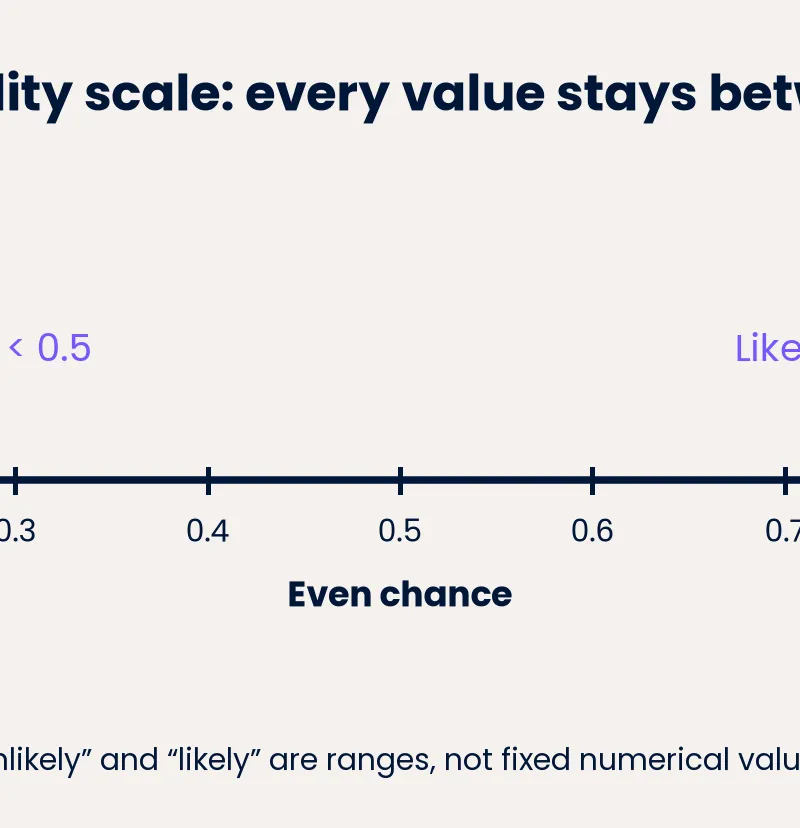
Probability measures how likely an event is. A numerical probability cannot be less than 0 or greater than 1. An impossible event has probability 0; a certain event has probability 1. An even chance has probability 0.5, equivalent to 1/2 or 50%.
Values between 0 and 0.5 describe unlikely events; values between 0.5 and 1 describe likely events. These words describe ranges, not fixed numerical values: unlikely does not always mean 0.25. A probability of 0.02 and a probability of 0.4 are both below an even chance, but 0.02 describes a much less likely event.
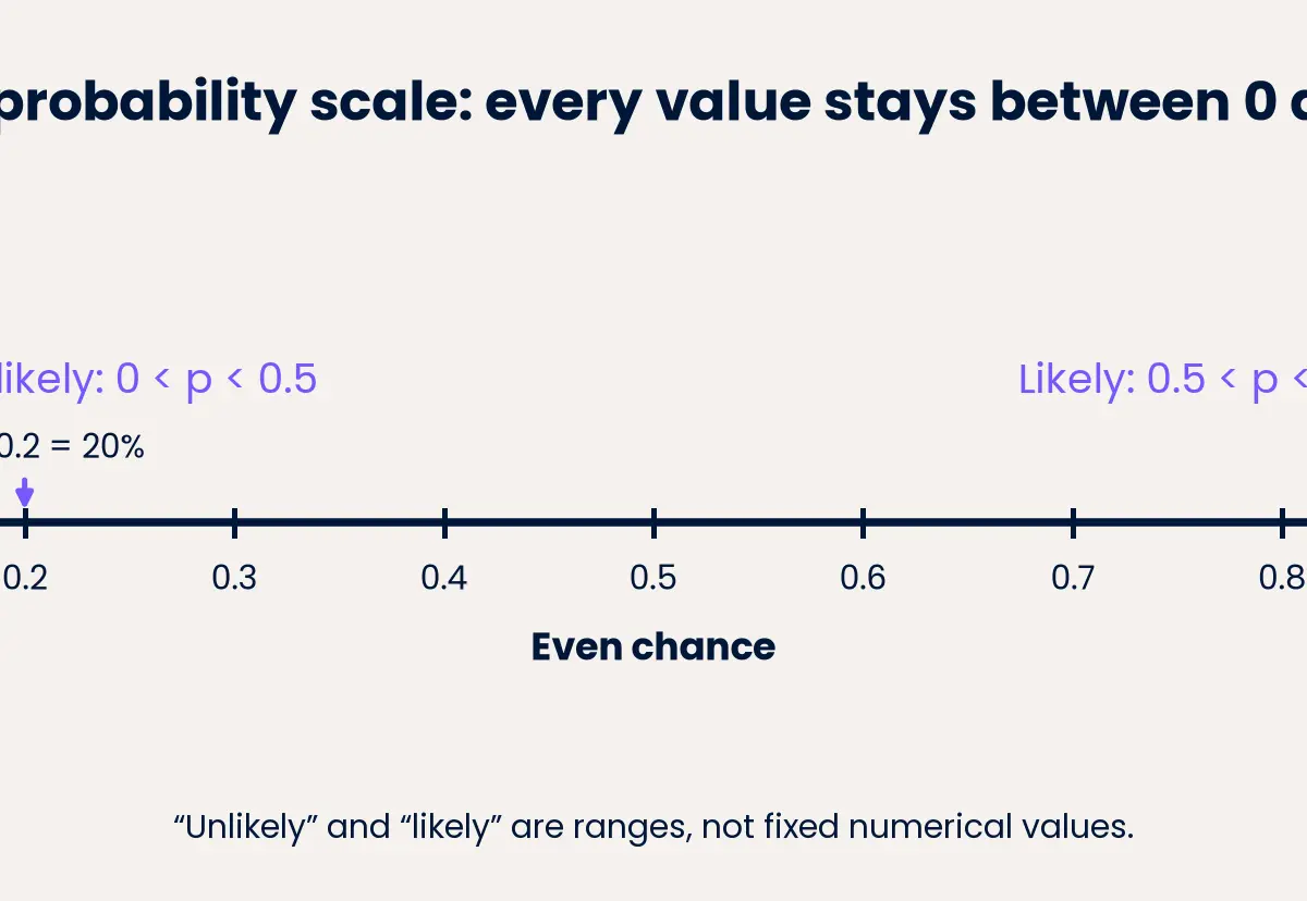
Example: A probability of 1/5 is 0.2. On a 10 cm scale running from 0 to 1, put the arrow 0.2 × 10 = 2 cm from 0. It belongs well to the left of the midpoint. Measure the full printed scale if necessary; never assume it is 10 cm long.
Cover and recall: What are the three exact anchor values? Then explain where 0.7 belongs without using the image. Credit given for a numerical probability requires a number: the word “certain” alone does not answer “Write down the probability”.
Concept 2: Accepted notation and careful conversion
Write probabilities as fractions, decimals or percentages. For example, 3/4 = 0.75 = 75%. The expressions 3:4 and “3 to 1” are ratios or odds, not the required probability notation. “1 in 4” describes a chance informally, but use 1/4 in an examination answer. Pearson's published marking guidance explicitly requires a fraction, percentage or decimal. 3
Remember the percentage sign. The numerical probability is 0.37, not 37; the percentage probability is 37%, not 0.37%. Prefer an exact fraction when the decimal recurs: write 1/6 rather than an unnecessarily rounded estimate. Unless a question specifies otherwise, Pearson's general guidance expects decimal equivalents to at least two decimal places, except exact tenths. Keep full values during intermediate calculations. 3
Why this works: “Per cent” means “out of 100”, so dividing a percentage by 100 converts it into the 0–1 scale. Probability has no physical unit. Do not attach centimetres, seconds or pounds to a probability, even when those units appear in the context.
Concept 3: Theoretical probability needs equally likely outcomes
Theoretical probability comes from a model. When all elementary outcomes are equally likely, divide the number of favourable outcomes by the total number of possible outcomes. “Favourable” simply means satisfying the named event, not necessarily a desirable result.
Example: A fair six-sided die has six equally likely outcomes. Three are even: 2, 4 and 6. Therefore P(even) = 3/6 = 1/2. For P(6), only one outcome qualifies, giving 1/6. Count carefully before you divide.
The fair-model assumption is essential. A spinner with four differently sized sectors does not give each sector probability 1/4 merely because there are four sectors. A drawing pin has two named landing outcomes, but its shape does not justify treating them as equally likely. Use experimental evidence instead unless a justified model is supplied.
What if? If a die is loaded, the outcomes 1 to 6 still exist, but counting them equally no longer produces its actual probabilities. The fair-die value remains a useful benchmark for investigating possible bias.
Concept 4: Relative frequency estimates probability from trials
A trial is one repetition of an experiment. The frequency of an event is the number of trials in which it occurs. Its relative frequency is that event frequency divided by the total number of trials.
Example: A drawing pin lands point up 37 times in 100 drops. Its relative frequency is 37/100 = 0.37. This is an estimate of P(point up) under those experimental conditions. It is not proof that the true probability is exactly 0.37.
If point up and point down are the only possible outcomes, point down occurs 100 − 37 = 63 times. Its relative frequency is 63/100 = 0.63. The two relative frequencies add to 1 because every drop belongs to exactly one of those categories.
Use successes over trials as your memory hook. In a frequency table, the denominator is normally the sum of all relevant outcome frequencies, not the number of categories. With zero trials, relative frequency is undefined because division by zero is not allowed.
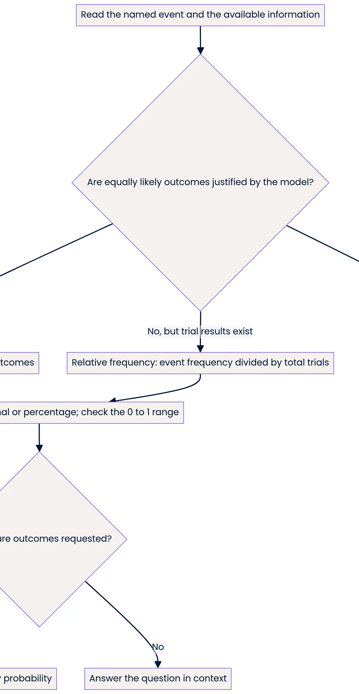
Cover and recall: Without looking, explain why 100/37 cannot be a probability. The event occurred in only some trials, so its frequency cannot exceed the total. Reversing the fraction creates a value above 1.
Concept 5: Compare estimates fairly and discuss possible bias
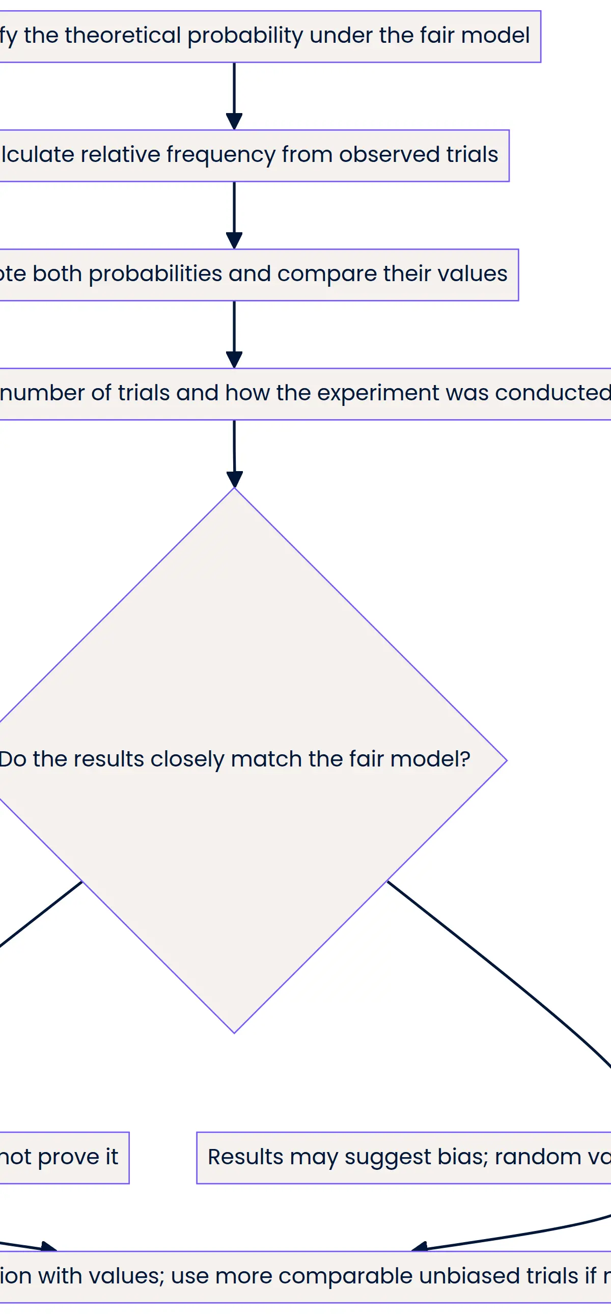
A fair coin has theoretical probability P(heads) = 0.5. If it produces 68 heads in 100 tosses, its relative frequency is 0.68. State both values and their direction: 0.68 is greater than 0.5. Then interpret the comparison: these results suggest a possible bias towards heads, although random variation could also cause a difference.
Do not claim that any difference proves bias. A fair coin need not give exactly 50 heads in 100 tosses. Equally, an experimental result of exactly 0.5 does not prove a coin is fair. A sensible conclusion uses “suggests”, “appears” or “is consistent with” and refers to the evidence.
A difference of 0.18 is 18 percentage points when comparing 68% with 50%. It is not automatically an 18% relative increase. For this topic, quoting the two probabilities and saying which is larger is usually the clearest comparison.
Examiner sentence frame: “The relative frequency is ___, compared with the theoretical probability ___; it is higher/lower, so the results suggest ___.” Add an appropriate caution when the question asks whether a claim is justified. Statistical significance tests and confidence intervals are not required for this P3 guide.
Concept 6: More trials usually improve reliability, not certainty
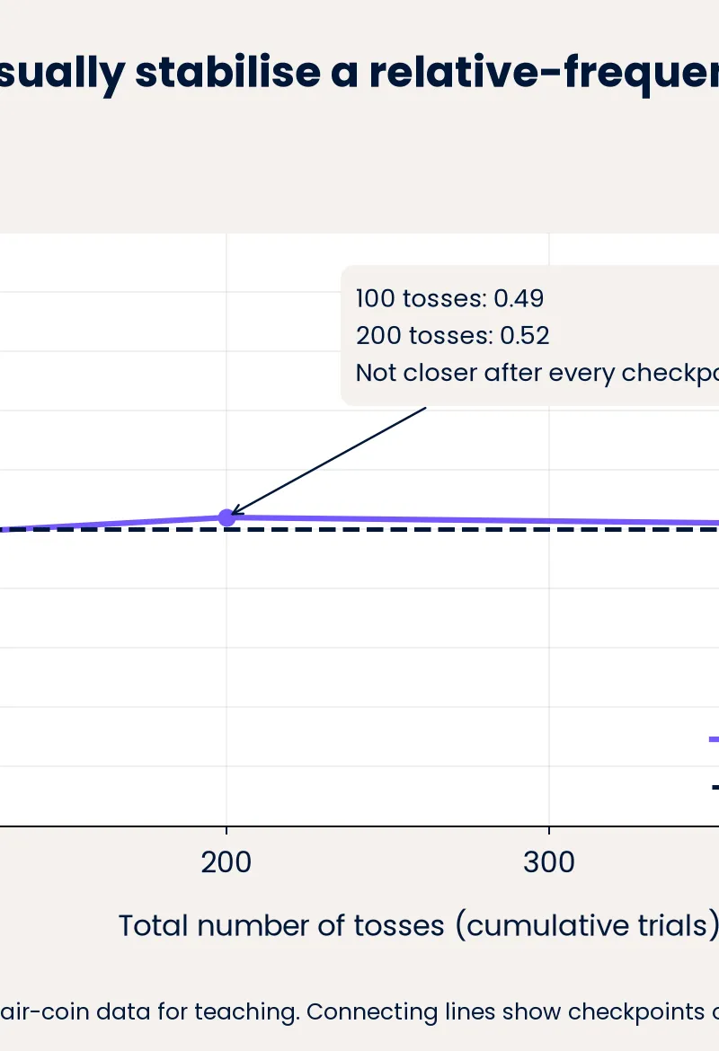
For repeated, comparable trials conducted without systematic sampling or recording bias, relative frequencies tend to settle towards the underlying probability as the number of trials grows. For a genuinely fair object, that underlying probability matches the fair theoretical model. This is the P5 connection. 1
The estimate does not have to get closer after every additional trial. It can move away temporarily. “Usually more reliable” does not mean “guaranteed correct”. Nor does a large experiment repair a faulty method: always starting a spinner in a particular way may distort results even after thousands of trials.
Example: Estimate A uses 10 coin tosses; estimate B uses 200 comparable tosses. B is usually more reliable because it is based on 200 trials rather than 10, reducing the influence of random fluctuations. Name the actual trial numbers in your explanation; “because it is bigger” is ambiguous.
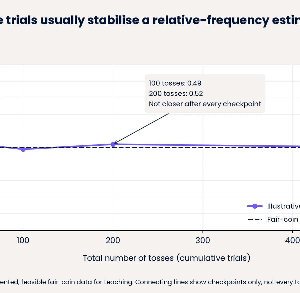
The illustration uses cumulative fair-coin data. Its points are (10, 0.70), (20, 0.55), (50, 0.52), (100, 0.49), (200, 0.52) and (500, 0.502). Notice the movement away from 0.5 between 100 and 200 trials. The overall stabilisation is not a promise of steady improvement.
Concept 7: Pool results using totals, not an unweighted average
When combining separate batches from the same experiment under comparable conditions, add successes and add trials. Then divide the combined successes by the combined trials.
Example: A pin lands point up 7 times in 20 drops, then 37 times in a further 100 drops. The pooled estimate is (7 + 37)/(20 + 100) = 44/120 = 11/30. Averaging 0.35 and 0.37 gives 0.36, which wrongly gives the small and large batches equal weight.
Read “further” carefully. If a table reports cumulative totals after 20 and 100 drops, the final total already includes the first 20. Use the final row rather than adding overlapping totals. Pooling also needs comparable conditions: changing the pin or landing surface could change the underlying probability.
Concept 8: Expected frequency is a prediction, not an observed count
Multiply the probability by the number of future trials to obtain an expected frequency. Use a theoretical probability for a justified fair model, or an estimated probability when experimental evidence is the appropriate basis.
Example: Using the pin estimate 0.37, the expected number of point-up landings in 200 further drops is 200 × 0.37 = 74. Write “about 74” or “an expected frequency of 74”, not “it will definitely land point up 74 times”.
The relative expected frequency is the expected count divided by trials: E/n = p. It equals the model probability. In contrast, the observed relative frequency f/n can differ because experiments fluctuate.
An expected frequency can be non-integer. A fair die has an expected 10 × 1/6 = 5/3 sixes in 10 rolls. That is a long-run average prediction, not an instruction to roll a fractional six. Follow any rounding instruction in the question; do not round the probability prematurely.
Mathematical Relationships
Must memorise: For equally likely outcomes, P(A) = number of outcomes satisfying A ÷ total number of possible outcomes. Here A names the event. Use this only when the equally likely assumption is justified.
Must memorise: Relative frequency r = f/n, where f is the observed event frequency and n > 0 is the total number of trials. Estimated probability P̂(A) = r. The hat means “estimated”; it does not mean the value is exact.
Must memorise: Expected frequency E = np, where n is the number of future trials and p is the appropriate theoretical or estimated probability. Rearrangements are p = E/n and n = E/p when the relevant denominator is non-zero. Expected frequency is a count prediction; probability is dimensionless.
Must memorise: P(not A) = 1 − P(A), and probabilities of an exhaustive set of mutually exclusive outcomes sum to 1. “Exhaustive” means all possibilities are included; “mutually exclusive” means they cannot occur together in a single trial. This is the P4 link.
Must memorise: Pooled relative frequency = (f₁ + f₂)/(n₁ + n₂) for separate comparable batches. Percentage probability = 100p%; decimal probability = numerical percentage ÷ 100. On a 0–1 line of length L, distance from 0 = pL. The distance has the same length unit as L.
Formula-sheet status: These relationships are not supplied on Pearson's 2026 Foundation formula sheet, so learn them. That sheet does include a separate addition rule for overlapping events, but it does not replace the formulas needed here. Check the sheet issued for your own examination series. 4
Graph and Data Skills
On a probability scale, locate the endpoints, convert to a decimal, and measure proportionally. On a relative-frequency graph, read the horizontal axis as total trials and the vertical axis as relative frequency. Use evenly spaced numerical scales and plot each ordered pair accurately. Join recorded checkpoints only to help show the trend; a connecting segment is not evidence of every unrecorded value.
For cumulative results, each frequency is a running total. Do not add the rows together. If a graph settles near 0.3 rather than a proposed fair-model value of 0.5, say it suggests a different underlying probability or a problem with the experiment, rather than declaring the fair model proven. Explain changes using the actual values read from the axes.
Practical Applications
Manufacturers estimate defect probabilities from samples; a sports coach estimates a player's scoring probability from recorded attempts. In each case, the data must be relevant to the future situation. A free-throw estimate from practice may not transfer unchanged to a pressured match.
There is no required practical assessment for this GCSE Mathematics topic. A useful optional experiment uses a coin or safe alternative to a sharp pin, a tray and a tally sheet. Define the outcomes, repeat the same randomised procedure, record every trial and calculate cumulative relative frequencies after agreed checkpoints. Avoid choosing which results to keep. Candidates may be asked to interpret results or explain how more trials improve an estimate, rather than describe a science practical.
Listen, Retrieve and Check
The ten-minute tutor episode follows: introduction 0:00–1:00; core concepts 1:00–6:00; exam tips 6:00–8:00; recall quiz 8:00–9:00; summary 9:00–10:00. Pause before answering each recall question. Attempt a worked example with the solution covered, compare your reasoning with the commentary, then retry it the next day. Connections earn credit when they answer the question, not merely because another topic is mentioned.
References
Worked Examples
4 worked examples — open one to explore the question and available guidance.
Practice Questions
Try the question, then reveal an answer plan or example response
State the probability of (a) an impossible event and (b) an event with an even chance. (2 marks)
Hint: Use the left endpoint and the midpoint of the probability scale.
A spinner lands on red 18 times in 60 spins. Calculate the relative frequency of red, then describe its likelihood using probability language. (3 marks)
Hint: Put red outcomes above total spins; compare the answer with 0.5.
A fair spinner has eight equal sectors numbered 1 to 8. (a) Calculate the probability of a multiple of 3. (2 marks) (b) Calculate the expected frequency of multiples of 3 in 120 spins. (2 marks)
Hint: List the qualifying numbers before using favourable outcomes over total outcomes.
A fair coin would have P(heads) = 0.5. An experiment produces 49 heads in 100 tosses. Calculate the relative frequency, then explain whether the results prove the coin is biased. (4 marks)
Hint: A fair model does not force an exact experimental split.
Two comparable pin-drop experiments give 4 point-up results in 10 drops and 72 in 200 drops. Calculate both estimates and state which is usually more reliable, giving a reason. (3 marks)
Hint: Reliability depends on comparable trial counts, not merely which decimal is larger.
Two separate comparable experiments give 6 successes in 20 trials and 45 successes in 100 further trials. Calculate the combined probability estimate, then use it to estimate the expected number of successes in 240 further trials. (5 marks)
Hint: Add successes and trials separately before dividing.
A cumulative table reports 7 heads after 10 tosses and 26 heads after 50 tosses. (a) Calculate the final relative frequency of heads. (2 marks) (b) Explain why adding the two rows is incorrect. (1 mark)
Hint: Cumulative means a running total.
Exam technique
How to turn what you know into marks
How to approach the question
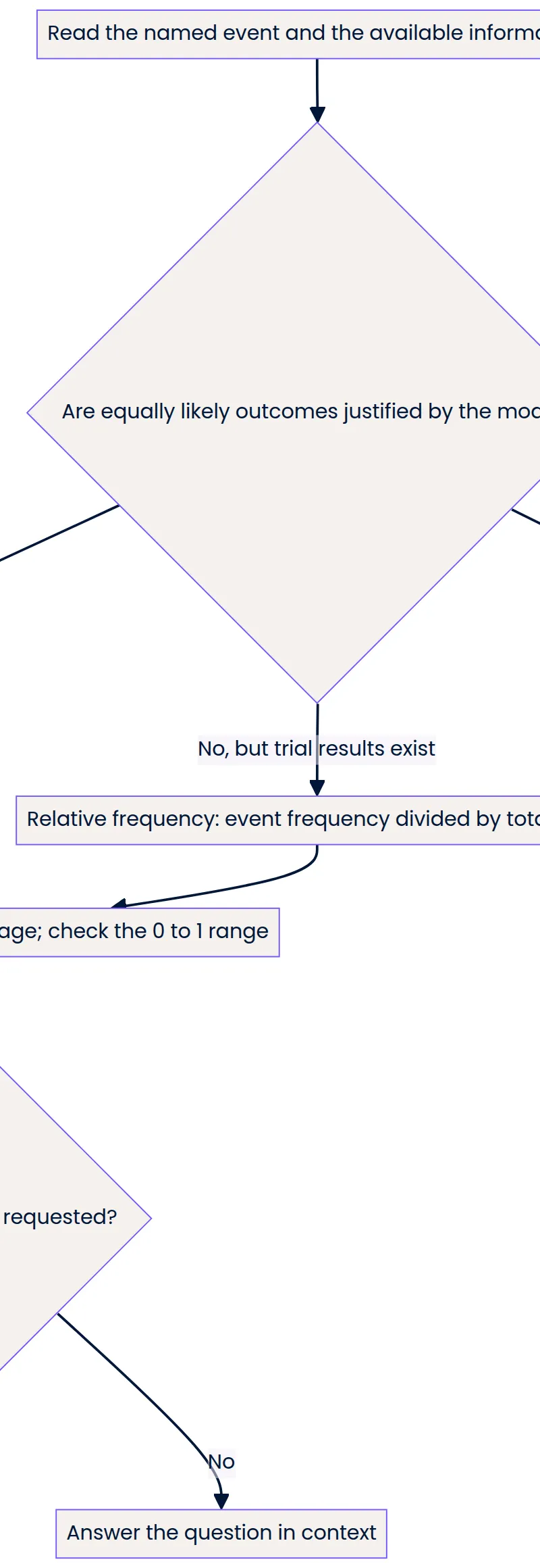
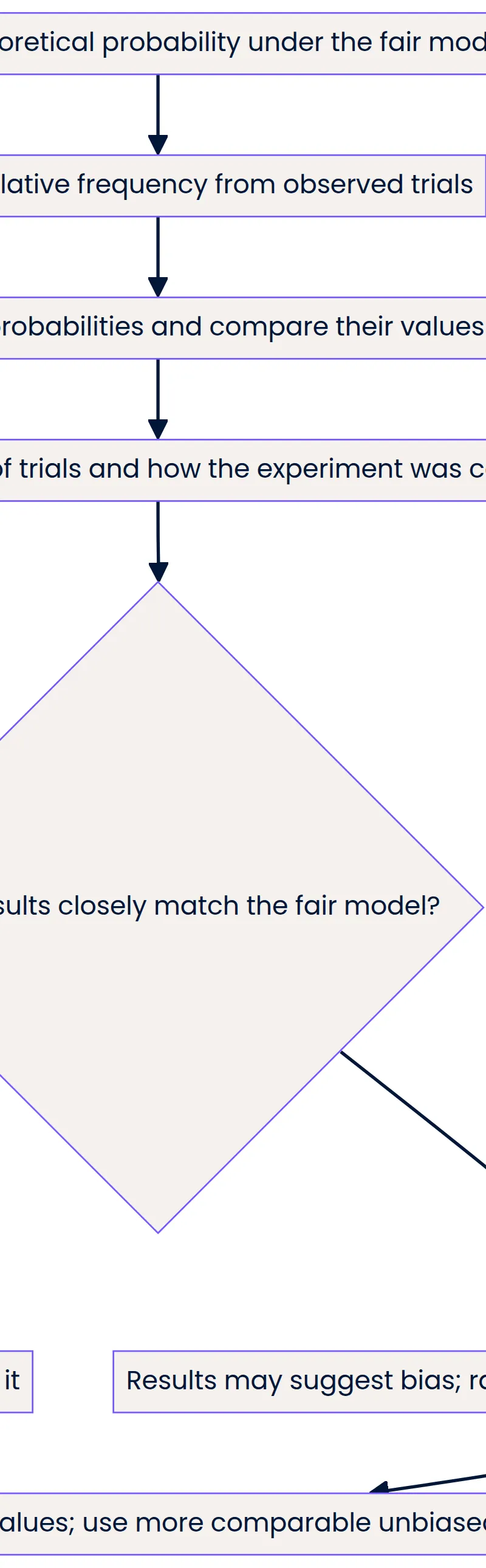
Identify the event and command word. Decide whether the information supports equally likely counting, an experimental estimate, a scale placement or an expected-frequency prediction. Check whether data rows are separate batches or cumulative. Carry out the calculation, check the 0–1 range for probabilities, and give a contextual reason if requested.
How to structure your answer
For a 1-mark give/state question, give the requested number or term. For a 2-mark calculation, show the correct fraction or operation and a correct final answer. For a comparison or explanation, quote both values and connect the conclusion to them using because. In multi-part 3–6-mark questions, answer every labelled part; there is no universal mark allocation shared by all probability questions.
Timing
Each paper is 90 minutes for 80 marks, equivalent to 1.125 minutes or 67.5 seconds per mark. As a flexible planning guide, aim for roughly 1 minute per mark so time remains for checking: about 3 minutes for 3 marks, 4 for 4 marks and 6–7 for 6 marks. This is revision advice, not an official time limit for each question.
Common pitfalls
- Reversing the fraction: write event frequency ÷ total trials and check the result is no more than 1.
- Writing 1:4 or 1 in 4 instead of 1/4: use accepted numerical probability notation.
- Omitting the percentage sign: 37% is a probability but 37 is not.
- Assuming two outcomes imply probability 1/2: equally likely outcomes need justification.
- Placing a scale arrow by eye: convert to a decimal and measure a proportional distance.
- Claiming every difference proves bias: compare with the fair benchmark and allow random variation.
- Claiming more trials guarantee a better estimate: say usually more reliable and require comparable, unbiased conditions.
- Averaging unequal batches or adding cumulative rows: pool separate counts, but use only the final cumulative totals.
- Rounding a probability too early: keep exact fractions or full calculator precision until the final instruction.
What the command words want
- Compare
- State both relevant probabilities or estimates and their relationship, such as 0.68 is greater than 0.5. Do not invent a requirement to list both similarities and differences when only one numerical comparison is requested.
- Explain
- Give a reason linked to the context, often using because. For reliability, quote the larger trial count and identify reduced random fluctuation.
- Describe
- Use appropriate likelihood or trend language. For a graph, name the pattern and support it with values where useful.
- Evaluate
- Assess the claim using the model, data, trial count and experimental limitations, then give a supported judgement without treating experimental evidence as automatic proof.
- Calculate
- Show the appropriate arithmetic and the result. Probability has no physical unit; an expected frequency counts outcomes. Follow any rounding instruction.
- State/Give
- Supply the requested answer briefly. If asked for a probability, write a number such as 1, not merely certain.
Watch or listen (optional)
Test your understanding of Probability: relate relative expected frequencies to theoretical probability, using appropriate language and the 0-1 probability scale
Active recall beats re-reading. Take an instant quiz now to test what you’ve learned and lock it into long-term memory.
7 days Premium · Then the free plan continues · No card, no charge