Big O Notation and Complexity Analysis Revision Notes
Subject: Computer Science | Level: A-Level | Exam Board: Edexcel
Master Big O Notation to predict how algorithms perform at scale. This guide breaks down complexity analysis into exam-focused chunks, showing you how to earn marks by comparing algorithms and justifying their efficiency.
Revision Notes & Key Concepts
Key Terms & Definitions
- Big O Notation
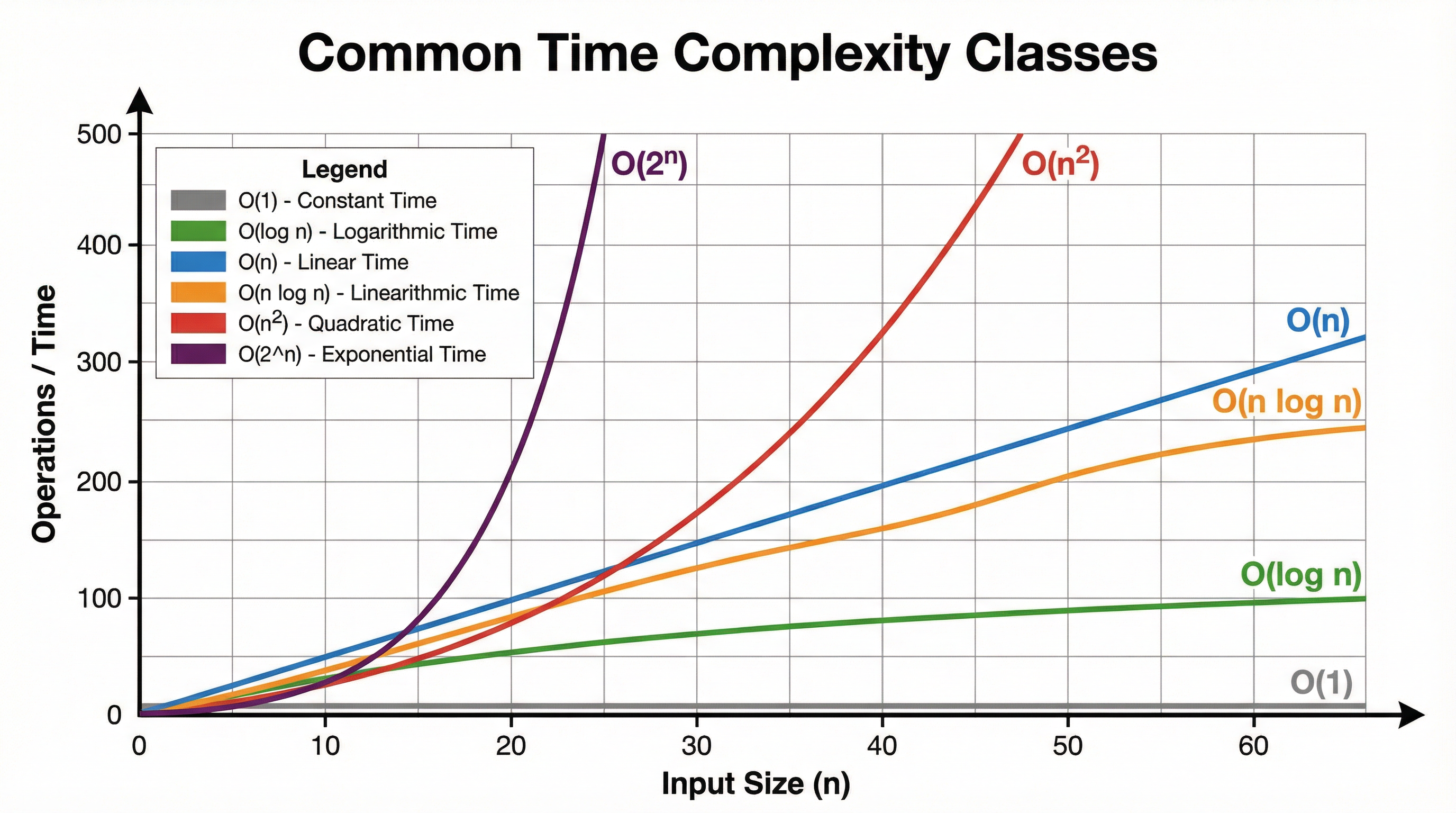
- A mathematical notation used to describe the limiting behavior of a function when the argument tends towards a particular value or infinity, used in computer science to classify algorithms according to their running time or space requirements.
- Time Complexity
- A measure of the amount of time an algorithm takes to run as a function of the length of the input.
- Space Complexity
- A measure of the amount of memory space an algorithm requires as a function of the length of the input.
- Worst-Case Scenario
- The input scenario for an algorithm that causes it to take the longest amount of time or consume the most resources.
- Dominant Term
- The term in a complexity expression that grows the fastest as the input size *n* increases. In Big O notation, all lower-order terms and coefficients are ignored.
- In-place Algorithm
- An algorithm that transforms input using no auxiliary data structure. The amount of extra space required is constant, i.e., O(1).
Worked Examples
Worked Example
Question: A sorting algorithm contains the following nested loops. Analyse the time complexity of this algorithm and express it using Big O notation. Justify your answer. (4 marks)
Solution: **Step 1: Analyse the outer loop.** The outer loop `for i from 0 to n-1` executes *n* times.\n**Step 2: Analyse the inner loop.** The inner loop `for j from 0 to n-1` also executes *n* times for *each* iteration of the outer loop.\n**Step 3: Calculate total operations.** The total number of times the inner comparison `if data[j] > data[j+1]` is executed is n * n = n². \n**Step 4: Express in Big O notation.** The dominant term is n². Therefore, the time complexity is **O(n²)**.
Worked Example
Question: Explain why the time complexity of a binary search algorithm is O(log n). (3 marks)
Solution: **Step 1: Describe the core process.** A binary search works on a sorted list. In each step, it compares the target value to the middle element of the current sublist.\n**Step 2: Link the process to the dataset size.** If the target is not the middle element, half of the list is discarded. The search then continues on the remaining half.\n**Step 3: Explain the logarithmic relationship.** Because the dataset is halved with each iteration, the number of operations required to find the element grows logarithmically with the size of the list, *n*. This means the time complexity is **O(log n)**.
Worked Example
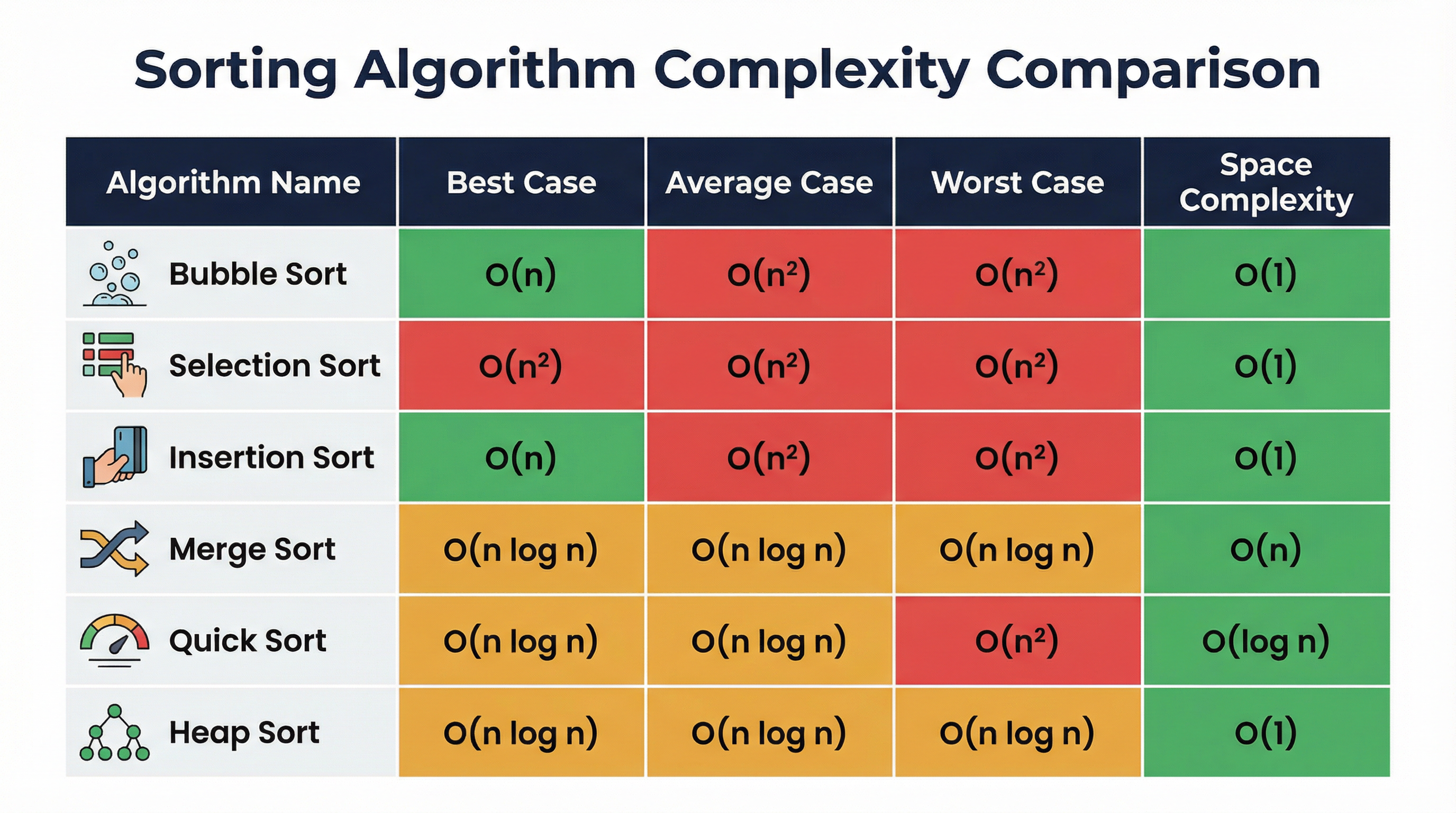
Question: Compare the time and space complexity of Merge Sort and Quicksort. (6 marks)
Solution: **Time Complexity Comparison (Average Case):**\n- Both Merge Sort and Quicksort have an average-case time complexity of **O(n log n)**. This makes them both highly efficient for large datasets.\n\n**Time Complexity Comparison (Worst Case):**\n- Merge Sort's worst-case time complexity is also **O(n log n)**, making its performance very consistent.\n- Quicksort, however, has a worst-case time complexity of **O(n²)**. This occurs when pivot selection is poor (e.g., on an already sorted list), leading to unbalanced partitions.\n\n**Space Complexity Comparison:**\n- Merge Sort has a space complexity of **O(n)** because it requires auxiliary arrays to merge the sorted sublists.\n- Quicksort has a better space complexity of **O(log n)** on average, as it performs the sort in-place and the memory usage is determined by the depth of the recursion stack.
Practice Questions
Question: What is the time complexity of accessing the 5th element in an array of size 10,000? Justify your answer. (2 marks)
Answer:
Question: An algorithm has a time complexity of O(n³). If it takes 2 seconds to run for an input of size n=100, estimate how long it will take for an input of size n=200. (3 marks)
Answer:
Question: A developer uses a recursive function to calculate the nth Fibonacci number. Analyse the time complexity of this naive recursive approach. (4 marks)
Answer:
Question: Why is it important to consider the worst-case complexity of an algorithm? Give an example. (3 marks)
Answer:
Question: Explain why an algorithm with O(n) space complexity may be unsuitable for an embedded system. (2 marks)
Answer: