Histograms

Overview

Histograms are a fundamental tool in statistics for representing grouped continuous data, but they are a significant step up from simple bar charts. For the OCR GCSE Further Mathematics exam, a solid understanding of histograms is essential, as questions frequently test the core principle that area is proportional to frequency. Unlike bar charts where the height of the bar is the key measure, in histograms, it is the area that tells the story. This topic is not just about drawing graphs; it is about interpreting them, solving problems where information is missing, and linking the visual representation of data to statistical calculations like the mean. Candidates who confuse histograms with bar charts invariably lose marks, so mastering the concept of frequency density is non-negotiable. Typical exam questions will involve constructing a histogram from a table, calculating frequencies from a given histogram (often without a scale on the vertical axis), and estimating the mean from the diagram.

Key Concepts

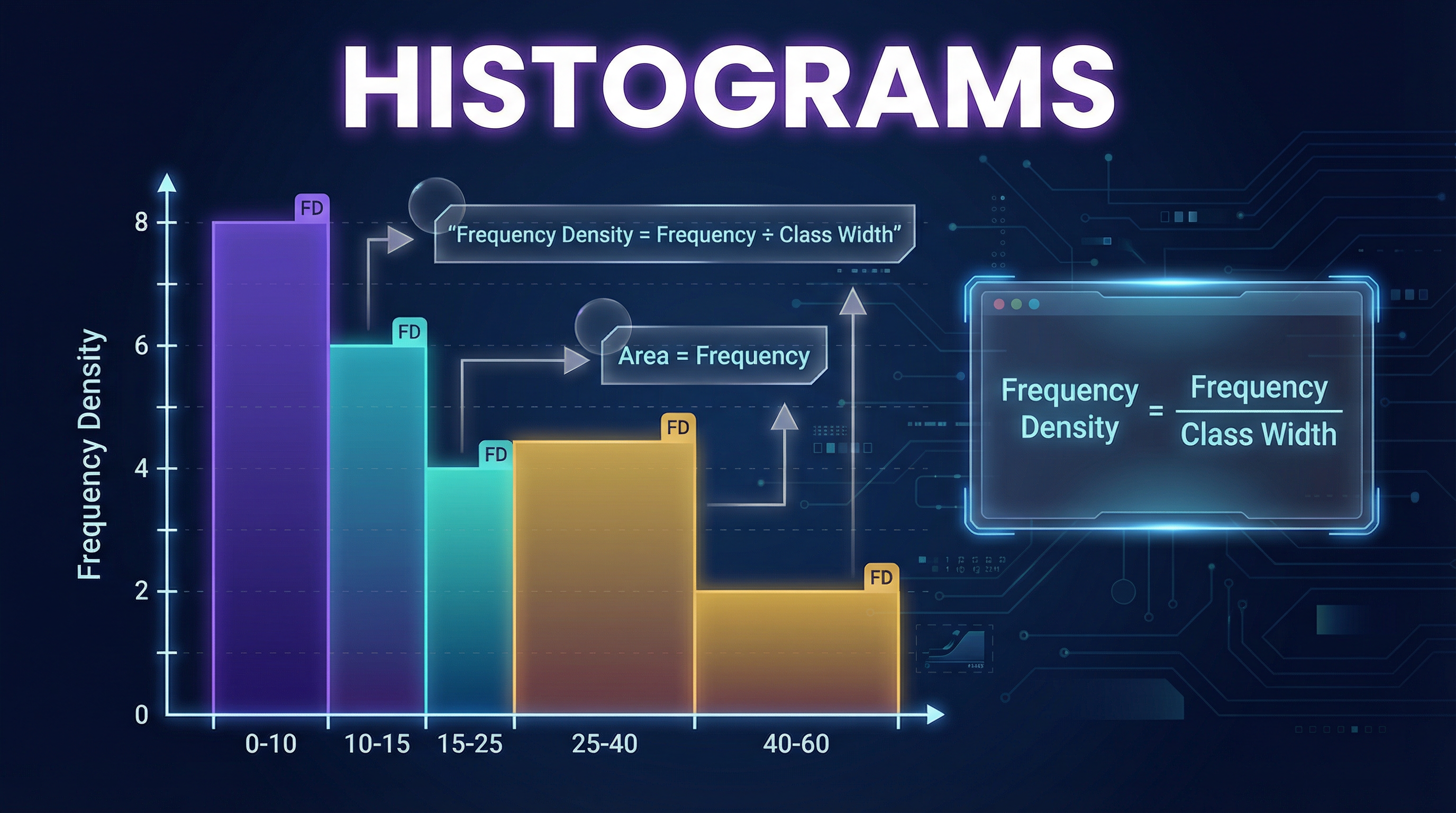
Concept 1: Frequency Density is Key

The single most important concept is Frequency Density (FD). Because the class intervals in a histogram can have unequal widths, plotting frequency directly on the vertical axis would create a misleading picture. A wide bar with a low frequency could look more significant than a narrow bar with a high frequency. To correct for this, we calculate the frequency density, which standardises the frequency per unit of width.

Example: Imagine two classes. Class A has a width of 10 and a frequency of 20. Class B has a width of 5 and a frequency of 20. If we just plotted frequency, the bars would be the same height, which is misleading because the data in Class B is twice as concentrated. By calculating frequency density (FD = F/CW), Class A has an FD of 2, while Class B has an FD of 4. The histogram bar for Class B will be twice as high, accurately reflecting the denser data.

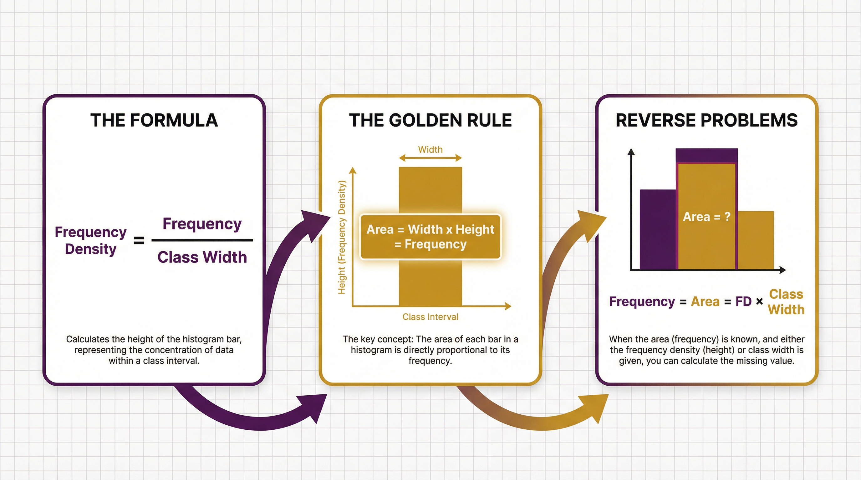
Concept 2: Area = Frequency

This is the golden rule that underpins all histogram calculations. The area of each bar is directly proportional to the frequency of that class. In the simplest case, the area is the frequency.

• Area = Class Width × Frequency Density
• Since Frequency Density = Frequency / Class Width
• Area = Class Width × (Frequency / Class Width) = FrequencyThis relationship is your tool for solving all types of histogram problems. If you are given a histogram and need to find the frequency of a certain bar, you simply calculate its area.

Mathematical/Scientific Relationships

The core formulas for histograms are:

1. Frequency Density = Frequency ÷ Class Width (Must memorise)

   • FD = F / CW
   • Use this when you have a frequency table and need to find the heights of the bars to draw the histogram.

2. Frequency = Frequency Density × Class Width (Must memorise)

   • F = FD × CW
   • Use this when you are given a histogram and need to find the frequency of a specific bar by calculating its area.

3. Estimate of the Mean = Σ(f × x) / Σf (Given on formula sheet)

   • Σ means 'sum of'.
   • f is the frequency of each class (the area of the bar).
   • x is the midpoint of each class interval.
   • Use this to calculate the estimated mean from a completed frequency table derived from a histogram.

Practical Applications

Histograms are used everywhere to analyse the distribution of data. For example:

• Manufacturing: A factory might use a histogram to analyse the distribution of lengths of bolts produced by a machine. Bars clustered tightly around the target length indicate high precision, while a wide spread indicates a problem.
• Finance: Analysts use histograms to understand the distribution of daily stock returns. This helps in assessing the risk and volatility of an investment.
• Population Studies: Demographers use histograms to show the age distribution of a population, which is crucial for planning social services like schools and pensions."