Pearson Edexcel · A-Level · Mathematics
Probability
Probability is the mathematical framework for quantifying uncertainty and making predictions based on data. This topic is central to Edexcel A-Level Mathematics, testing your ability to translate real-world scenarios into precise mathematical models using set notation, conditional logic, and statistical distributions. Mastering probability is essential for success in the exam and provides a foundation for further study in STEM, finance, and the social sciences.
- 8 min read
- 4 worked examples
- 5 practice questions
- 10 key terms
Study Notes

Overview
Probability is a cornerstone of A-Level Mathematics, forming the bedrock of statistics and data analysis. It is the mathematical language we use to quantify uncertainty and make informed predictions about the world. For Edexcel A-Level candidates, this topic is not just about calculating the chances of rolling a six; it's a rigorous test of logical reasoning, problem-solving, and the ability to translate complex, real-world scenarios into precise mathematical models. Examiners frequently use probability to assess a candidate's ability to connect different areas of mathematics, from set theory to calculus. A strong grasp of probability is essential for success in the statistics component of the exam and provides a vital foundation for further study in STEM, finance, and social sciences. Typical exam questions range from short, 2-mark calculations to extended, multi-part problems that require you to select and justify an appropriate probability distribution.
Key Concepts
Concept 1: Set Notation and Venn Diagrams
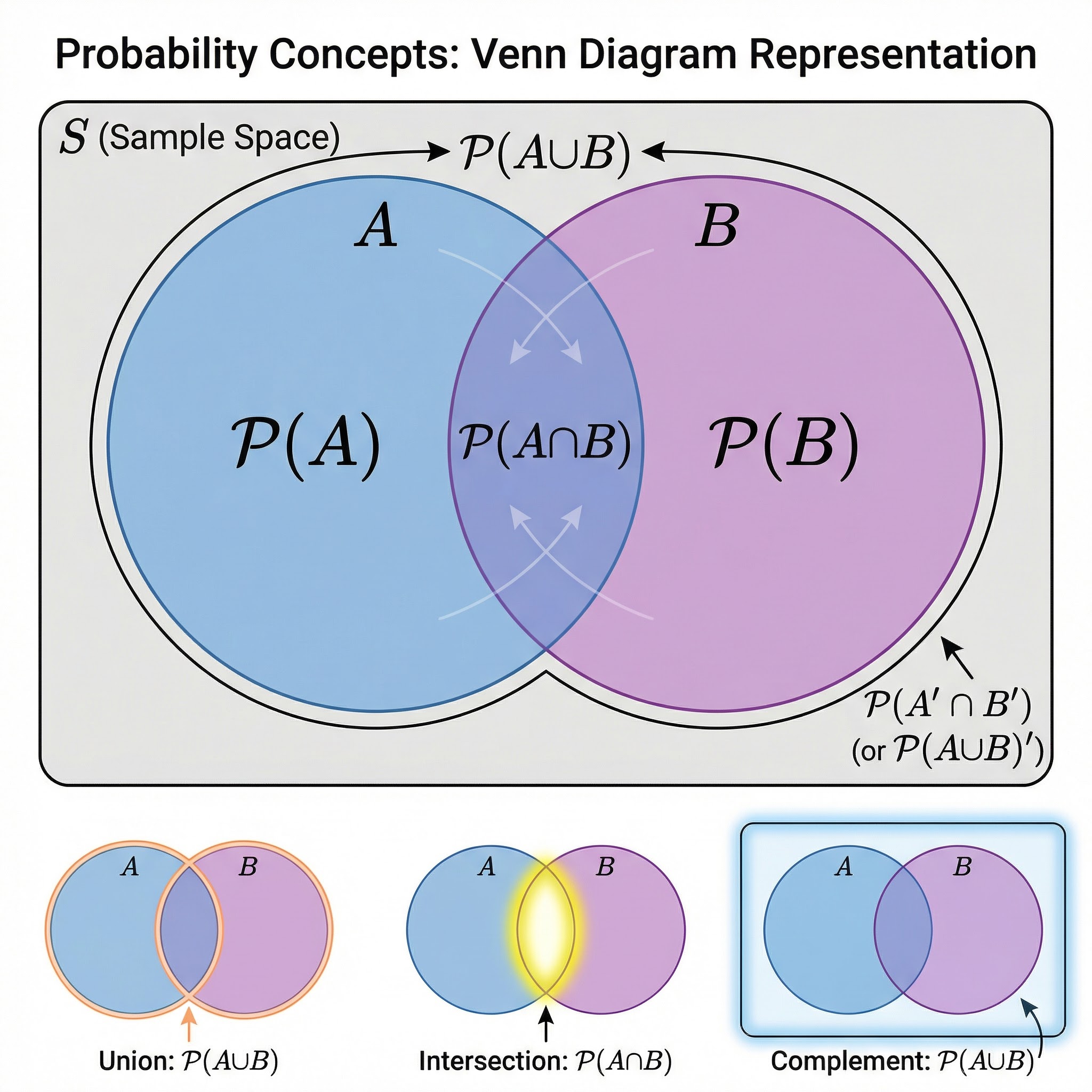
At its heart, probability is built on the principles of set theory. An event is simply a set of outcomes, and we use specific notation to describe the relationships between these events. Mastering this language is the first step to earning marks.
- Sample Space (S or ξ): The set of all possible outcomes.
- Event (A, B, etc.): A subset of the sample space.
- Union (A ∪ B): The event that A or B or both occur. Think of this as the total area covered by both sets.
- Intersection (A ∩ B): The event that both A and B occur simultaneously. This is the overlapping region of the sets.
- Complement (A'): The event that A does not occur. This is everything in the sample space outside of A.
Venn diagrams are powerful tools for visualizing these relationships. They allow you to turn abstract probabilities into a concrete picture, which can make complex problems much easier to solve. Credit is often given for drawing a clear, well-labelled Venn diagram.
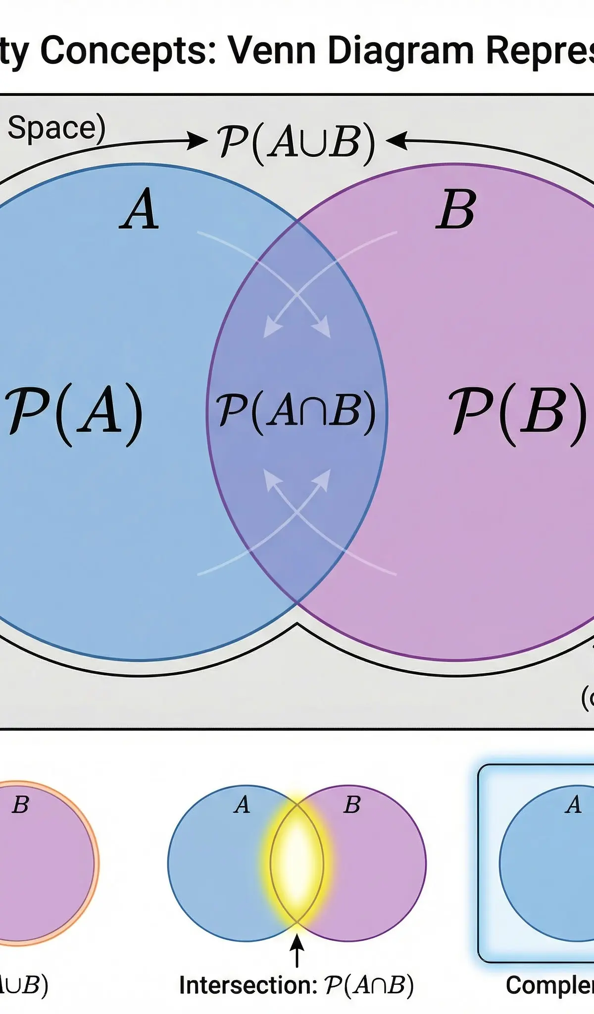
Example: In a class of 30 students, 15 study French (F), 20 study Spanish (S), and 5 study neither. To find how many study both, we can use the formula: P(F ∪ S) = P(F) + P(S) - P(F ∩ S). First, find the number of students who study at least one language: 30 - 5 = 25. So, 25 = 15 + 20 - |F ∩ S|. Solving this gives |F ∩ S| = 10. Ten students study both French and Spanish.
Concept 2: Conditional Probability and Independence
Conditional probability is the probability of an event occurring, given that another event has already occurred. This is a frequent source of confusion, but the key is to recognise that the sample space has been reduced. The notation is P(A|B), read as "the probability of A given B".
Formula: P(A|B) = P(A ∩ B) / P(B)
This formula is your go-to for any conditional probability calculation. It essentially asks: of all the outcomes where B happened, what proportion of them were also A outcomes?
Independence is a special case. Two events are independent if the occurrence of one does not affect the probability of the other. For example, flipping a coin twice. The outcome of the first flip has no impact on the second.
Test for Independence: Events A and B are independent if and only if:
P(A ∩ B) = P(A) * P(B)
An equivalent test is P(A|B) = P(A).
Examiners will explicitly ask you to 'Show that' or 'Explain why' two events are or are not independent. You must perform the calculation and state your conclusion clearly. Never assume independence unless the context makes it obvious (e.g., sampling with replacement).
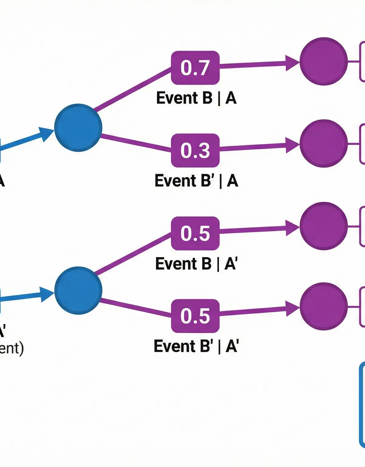
Concept 3: Tree Diagrams
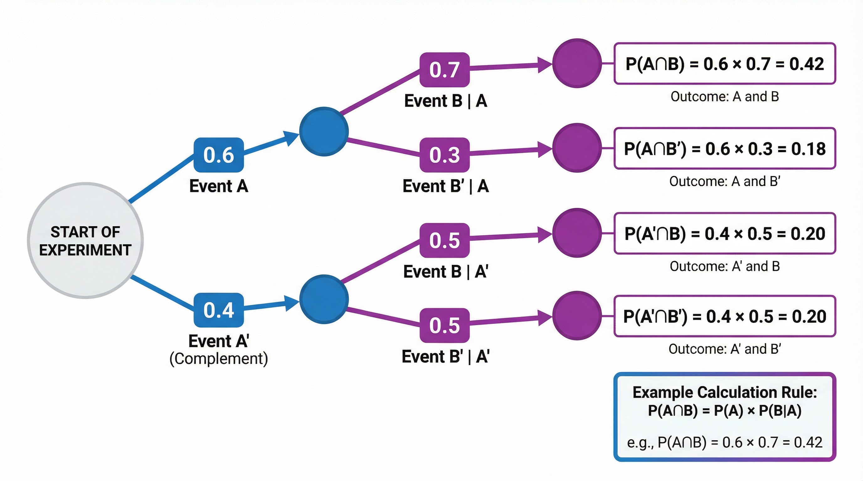
Tree diagrams are visual representations of multi-stage experiments. They are particularly useful for calculating probabilities when events occur in sequence. Each branch represents an outcome, and the probability of that outcome is written on the branch. To find the probability of a specific path through the tree, you multiply the probabilities along that path. To find the probability of multiple paths (e.g., "at least one success"), you add the probabilities of each relevant path.
Key Rule: Multiply along the branches, add between the branches.
Concept 4: Probability Distributions
A probability distribution is a function that describes the likelihood of all possible outcomes for a random variable. For A-Level, you need to master two key distributions.
**1. The Binomial Distribution: X ~ B(n, p)**Use the Binomial distribution when you are counting the number of 'successes' in a fixed number of independent trials.
- n: The number of trials (must be fixed).
- p: The probability of success on a single trial (must be constant).
- The trials must be independent.
- There are only two outcomes for each trial (success/failure).
Your calculator is essential here. You need to be proficient with the 'Binomial PD' (for P(X=x)) and 'Binomial CD' (for P(X≤x)) functions.
Example: A biased coin with P(Head) = 0.6 is flipped 10 times. The probability of getting exactly 7 heads is a Binomial problem with n=10, p=0.6, x=7. You would use Binomial PD on your calculator.
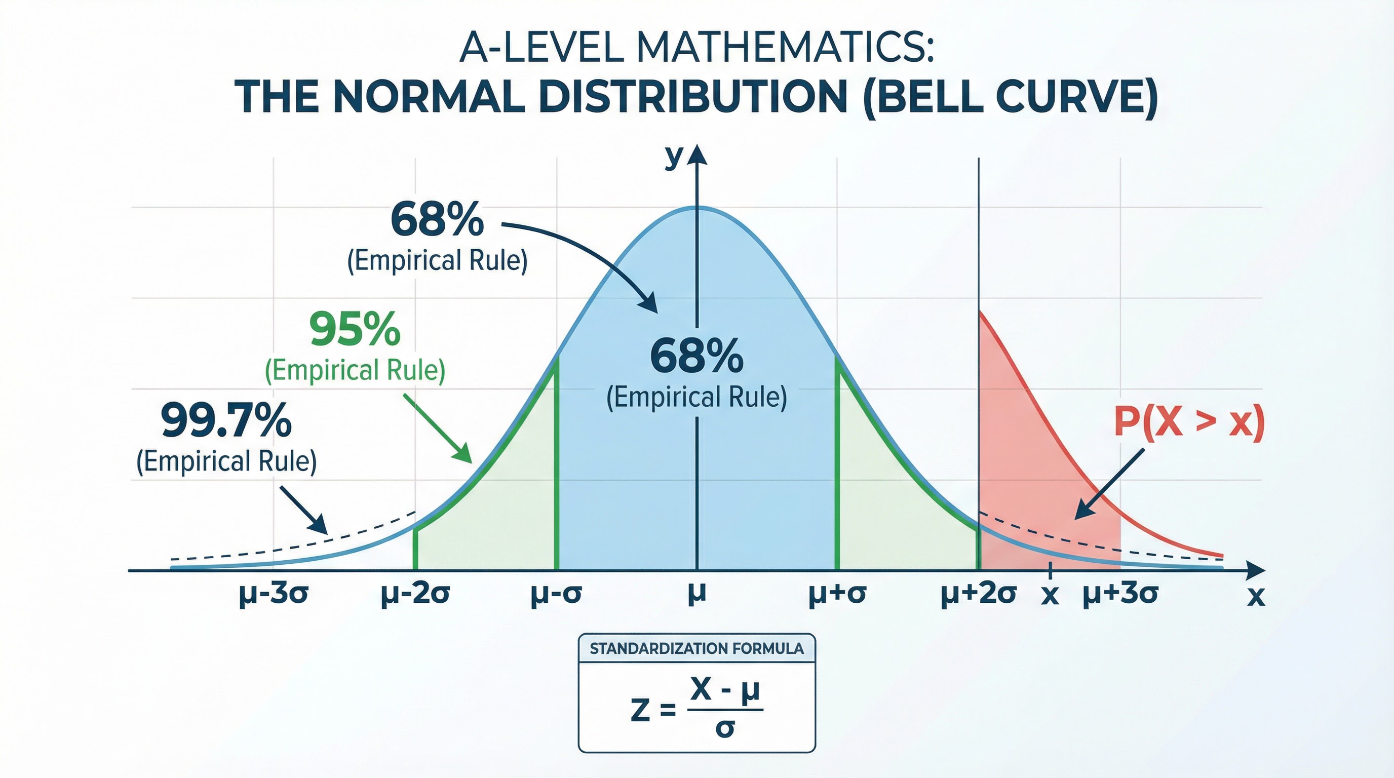
**2. The Normal Distribution: X ~ N(μ, σ²)**The Normal distribution is a continuous distribution represented by the classic 'bell curve'. It is arguably the most important distribution in statistics.
- μ (mu): The mean of the distribution (the peak of the curve).
- σ² (sigma-squared): The variance of the distribution (a measure of spread). Remember that the standard deviation, σ, is the square root of the variance.
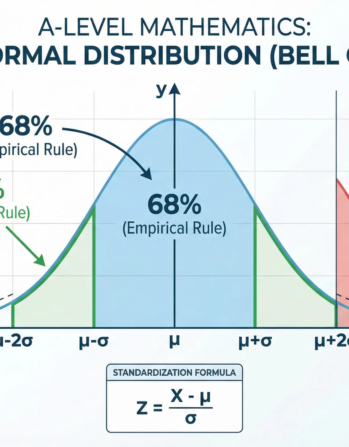
Calculations are done using your calculator's 'Normal CD' function. A crucial skill is standardisation, which converts any Normal variable into the standard Normal distribution Z ~ N(0, 1).
Standardisation Formula: Z = (X - μ) / σ
This is vital when you need to find an unknown mean or standard deviation, as you will use the Inverse Normal function on your calculator to find a Z-value and then solve for the unknown.
Concept 5: Continuity Corrections
When you approximate a discrete Binomial distribution with a continuous Normal distribution, you must apply a continuity correction. This adjusts the boundaries to account for the fact that you're using a continuous curve to model discrete values.
- For P(X = k), use P(k - 0.5 < X < k + 0.5)
- For P(X ≥ k), use P(X > k - 0.5)
- For P(X ≤ k), use P(X < k + 0.5)
- For P(X > k), use P(X > k + 0.5)
- For P(X < k), use P(X < k - 0.5)
Failing to apply the continuity correction when required will lose you marks.
Mathematical/Scientific Relationships
Formulas You Must Know:
| Formula | Status | Use |
|---|---|---|
| P(A ∪ B) = P(A) + P(B) - P(A ∩ B) | Given on formula sheet | Addition rule for probabilities |
| P(A | B) = P(A ∩ B) / P(B) | Must memorise |
| P(A ∩ B) = P(A) * P(B) | Must memorise | Test for independence |
| P(X=r) = (nCr) * p^r * (1-p)^(n-r) | Given on formula sheet | Binomial probability (but use calculator) |
| Z = (X - μ) / σ | Must memorise | Standardisation for Normal distribution |
| E(X) = np | Given on formula sheet | Expected value for Binomial |
| Var(X) = np(1-p) | Given on formula sheet | Variance for Binomial |
Practical Applications
Probability isn't just an abstract concept; it's used everywhere:
- Finance: To model stock prices and assess investment risk.
- Insurance: To calculate premiums based on the likelihood of events like car accidents or house fires.
- Medicine: In clinical trials to determine the effectiveness of new drugs.
- Quality Control: In manufacturing to determine the probability of a product being defective.
- Weather Forecasting: To predict the chance of rain or snow.
Understanding these applications can help you make sense of exam questions that are set in a real-world context.
Listen to the Podcast

Visual Resources
3 diagrams and illustrations
Interactive Diagrams
2 interactive diagrams to visualise key concepts
Conceptual Flow Outline
Decision flowchart for choosing the correct probability method in Edexcel A-Level Mathematics
Conceptual Flow Outline
Process for testing whether two events are independent
Worked Examples
4 worked examples — open one to explore the question and available guidance.
Practice Questions
Test your understanding — click to reveal model answers
A fair six-sided die is rolled twice. Find the probability that the sum of the two rolls is 9.
Hint: List all the pairs of outcomes that give a sum of 9, then divide by the total number of possible outcomes.
In a group of 100 people, 60 like tea (T), 50 like coffee (C), and 20 like neither. (a) Draw a Venn diagram to represent this information. (2 marks) (b) Find the probability that a randomly selected person likes both tea and coffee. (2 marks)
Hint: Start by finding how many people like at least one drink, then use the addition rule to find the overlap.
A factory produces light bulbs. The probability that a bulb is defective is 0.02. A sample of 50 bulbs is taken. Using a suitable approximation, find the probability that fewer than 3 bulbs are defective.
Hint: This is a Binomial problem, but with large n you can approximate with a Normal distribution. Don't forget the continuity correction.
The masses of apples in a supermarket are normally distributed with mean 150g and standard deviation 20g. An apple is classified as 'large' if its mass is in the top 10% of all apples. Find the minimum mass for an apple to be classified as large.
Hint: You need to find the mass m such that P(X > m) = 0.10, which is the same as P(X < m) = 0.90. Use Inverse Normal.
Events A and B are such that P(A) = 0.6, P(B|A) = 0.4, and P(B|A') = 0.3. Find P(B).
Hint: Use the law of total probability: P(B) = P(B|A) × P(A) + P(B|A') × P(A').