OCR · A-Level · Physics
Course version: H556 · Version from Sept 2015
Stationary waves: (b) graphical representations of a stationary wave
A stationary wave can be represented graphically in two ways.
Checked against the OCR H556 specification (opens in a new tab) on .
- Point 3 of 8
- 4 key terms
Study notes
From the checked teaching notes for this specification point.
The idea
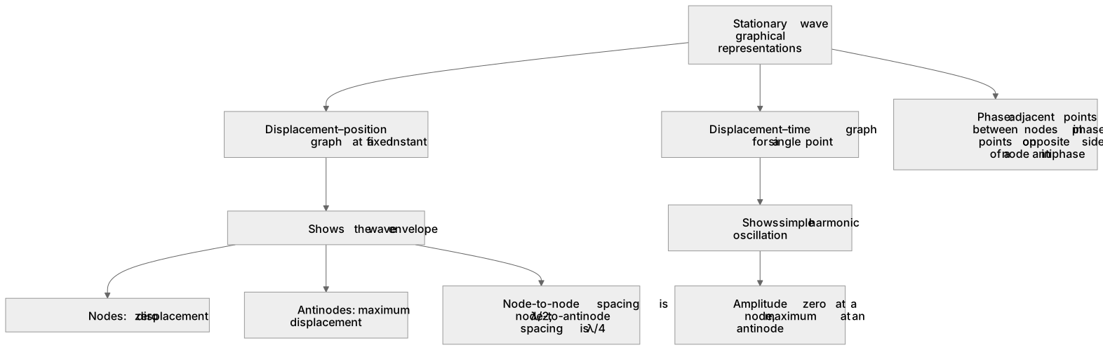
A stationary wave can be represented graphically in two ways. A displacement–position graph at a fixed instant shows the wave envelope: a sine or cosine curve with regularly spaced nodes and antinodes, where the curve crosses the axis at nodes and reaches maxima at antinodes. A displacement–time graph for a single point shows simple harmonic oscillation whose amplitude depends on the point's position: zero at a node, maximum at an antinode. Adjacent points between nodes oscillate in phase, while points on opposite sides of a node are in antiphase.
For example: On a string fixed at both ends, the fundamental mode has nodes at the ends and one antinode at the centre, and its displacement–position graph is a single half-sine curve.
What earns the marks
- A displacement–position graph at an instant shows the stationary wave envelope with nodes at zero displacement and antinodes at maximum displacement.
- A displacement–time graph for a chosen point shows simple harmonic oscillation with amplitude set by the point's position.
- Adjacent points between two nodes oscillate in phase; points on opposite sides of a node are in antiphase.
- Node-to-node spacing on the graph is λ/2 and node-to-antinode spacing is λ/4.
- The number of half-wavelengths fitting the boundary conditions identifies the mode of vibration.
Common mistakes and how to put them right
Reading a displacement–position graph as if the wave were travelling.
Put it right by noting that the envelope is fixed in space and only the displacements change with time.
Assuming all points on a stationary wave oscillate in phase.
Put it right by identifying phase differences between adjacent segments separated by nodes.
Confusing the amplitude of a point with the amplitude of the whole wave.
Put it right by stating that amplitude varies from zero at nodes to maximum at antinodes.
Exam tips
- Label nodes and antinodes on any sketch before interpreting the graph.
- Use the graph to read node-to-node spacing and convert to wavelength using λ = 2 × spacing.
- For displacement–time graphs, check the amplitude against the point's position on the envelope.
Try the lesson
The start of the Stationary waves: (b) graphical representations of a stationary wave lesson, made from checked teaching notes for this specification point.
Listen
A stationary wave can be represented graphically in two ways. A displacement–position graph at a fixed instant shows the wave envelope: a sine or cosine curve with regularly spaced nodes and antinodes, where the curve crosses the axis at nodes and reaches maxima at antinodes. A displacement–time graph for a single point shows simple harmonic oscillation whose amplitude depends on the point's position: zero at a node, maximum at an antinode. Adjacent points between nodes oscillate in phase, while points on opposite sides of a node are in antiphase. For example, on a string fixed at both ends, the fundamental mode has nodes at the ends and one antinode at the centre, and its displacement–position graph is a single half-sine curve. A strong answer earns marks for these points. A displacement–position graph at an instant shows the stationary wave envelope with nodes at zero displacement and antinodes at maximum displacement. A displacement–time graph for a chosen point shows simple harmonic oscillation with amplitude set by the point's position. Adjacent points between two nodes oscillate in phase; points on opposite sides of a node are in antiphase. Node-to-node spacing on the graph is λ/2 and node-to-antinode spacing is λ/4. A common slip: Reading a displacement–position graph as if the wave were travelling. Instead, noting that the envelope is fixed in space and only the displacements change with time. Exam tip: Label nodes and antinodes on any sketch before interpreting the graph.
See it
Key words
Say what each word means before you turn the card.
Displacement–position envelope
Try answering aloud or in your head before turning the card.
Displacement–time oscillation
Try answering aloud or in your head before turning the card.
Phase relationships between points
Try answering aloud or in your head before turning the card.
Modes and boundary conditions
Try answering aloud or in your head before turning the card.
See every definition
- Displacement–position envelope
- A graph at a fixed instant showing a sine or cosine curve with regularly spaced nodes and antinodes, crossing the axis at nodes and reaching maxima at antinodes.
- Displacement–time oscillation
- A graph for a single point showing simple harmonic oscillation whose amplitude depends on the point's position: zero at a node, maximum at an antinode.
- Phase relationships between points
- Adjacent points between nodes oscillate in phase, while points on opposite sides of a node are in antiphase.
- Modes and boundary conditions
- The number of half-wavelengths fitting the boundary conditions identifies the mode of vibration, such as the fundamental mode on a string fixed at both ends.
Label the diagram
Some boxes have lost their names. Pick the right name for each number.
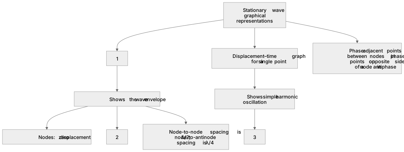
1Box 1
2Box 2
3Box 3
There is more to this lesson
The full lesson goes on to check your understanding and help you earn the marks. Create a free account to carry on, with your progress saved.
A week of Premium from your first lesson · Then the free plan continues · No card, no charge
Test your understanding of Stationary waves: (b) graphical representations of a stationary wave
Active recall beats re-reading. Take an instant quiz now to test what you’ve learned and lock it into long-term memory.
A week of Premium from your first lesson · Then the free plan continues · No card, no charge