Half-life — OCR GCSE Study Guide
Exam Board: OCR | Level: GCSE
Master radioactive half-life for your OCR GCSE Physics exam. This guide breaks down how to read decay graphs, perform calculations, and apply concepts to real-world scenarios like medical imaging, ensuring you can secure every mark available on this key topic.
## Overview
Radioactive half-life is a fundamental concept in nuclear physics that describes the statistical nature of radioactive decay. For your OCR GCSE exam, a thorough understanding is crucial as it is assessed through a combination of graphical analysis, numerical problems, and application-based questions. This topic explains why the activity of a radioactive sample decreases over time and provides a predictable way to measure this decay. It connects directly to concepts of atomic structure, isotopes, and the different types of radiation. Examiners typically ask candidates to determine half-life from a decay curve, calculate the remaining activity of a sample after a certain time, or evaluate the suitability of different isotopes for specific uses, such as in medicine or industry. Mastering the skills in this guide will equip you to tackle these questions with confidence.

## Key Concepts
### Concept 1: The Nature of Radioactive Decay
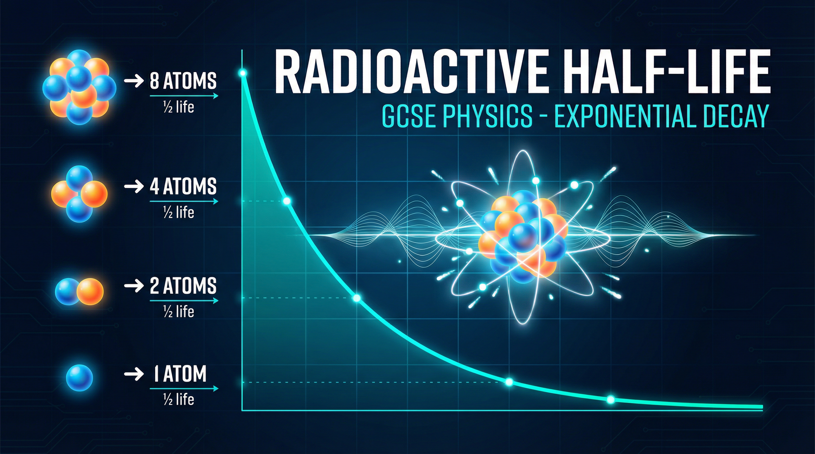
Radioactive decay is a **random process**. It is impossible to predict when a single unstable nucleus will decay. However, when dealing with a vast number of nuclei in a sample, the overall behavior becomes statistically predictable. This is the foundation of the half-life concept. The **activity** of a sample, measured in Becquerels (Bq), is the number of nuclei that decay per second. As the number of unstable nuclei decreases, the activity also decreases. This is not a linear process; it is an **exponential decay**. The rate of decay is always proportional to the number of remaining unstable nuclei.
**Analogy**: Imagine a box full of popcorn kernels being heated. You cannot predict which kernel will pop next, but you know that after a certain time, a large fraction will have popped. As time goes on, the rate of popping slows down because there are fewer unpopped kernels left. Radioactive decay works in the same way.
### Concept 2: Defining and Calculating Half-Life
Half-life (symbol: t) is formally defined as **the time taken for the number of undecayed radioactive nuclei in a sample to halve, OR the time taken for the activity of the sample to fall to half of its initial value.** Both definitions are accepted by examiners and are worth 1 mark.
This means that after one half-life, the activity is 1/2 of the original. After two half-lives, it is 1/4 of the original. After three half-lives, it is 1/8 of the original, and so on. The key is to identify the number of half-lives that have passed in a given time period.
**Example**: A sample of Cobalt-60 has a half-life of 5 years and an initial activity of 1200 Bq. To find the activity after 15 years:
1. Calculate the number of half-lives: Total time / Half-life = 15 years / 5 years = 3 half-lives.
2. Write out the decay chain explicitly:
- After 1 half-life (5 years): 1200 Bq -> 600 Bq
- After 2 half-lives (10 years): 600 Bq -> 300 Bq
- After 3 half-lives (15 years): 300 Bq -> 150 Bq
The final activity is 150 Bq. Showing this sequence is often required for a calculation mark.
### Concept 3: Graphical Representation of Decay
OCR frequently tests half-life using decay curves. These graphs plot Activity (y-axis) against Time (x-axis). The curve is always exponential, starting steep and becoming progressively shallower as it approaches zero.
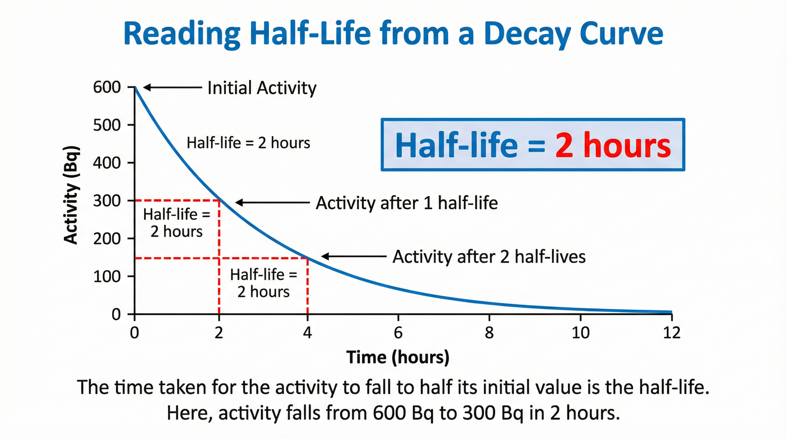
To determine the half-life from a graph, you MUST draw construction lines to receive method marks:
1. **Select a convenient starting activity** on the y-axis (e.g., 800 Bq).
2. **Halve this value** (e.g., 400 Bq).
3. **Draw a horizontal line** from this halved activity value on the y-axis across to the decay curve.
4. **Draw a vertical line** from the point of intersection on the curve down to the x-axis.
5. **Read the time** from the x-axis. This time is the half-life.
For full credit, it is good practice to repeat this process from a second point (e.g., from 400 Bq to 200 Bq) to confirm your value.
### Concept 4: Background Radiation
No measurement of radioactivity is complete without considering **background radiation**. This is the low-level ionising radiation that is always present in our environment from natural and man-made sources (e.g., cosmic rays, rocks, medical procedures). A Geiger-Muller tube will always detect this background count. Therefore, to get an accurate measurement of a source's activity, you must first measure the background count rate separately and then **subtract this value from all of your measurements** of the source.
**Exam Tip**: If a question provides a value for background radiation (e.g., 'The background count was 30 counts per minute'), it is a direct instruction to use it. Failure to subtract the background count before plotting a graph or calculating a half-life is a common error that will lose you marks.
## Mathematical/Scientific Relationships
The relationship between the number of half-lives (n), the total time elapsed (t), and the half-life (t_half) is:
n = t / t_half
This formula is **not given on the formula sheet** and must be understood, although it is more of a logical step than a formula to memorise.
The fraction of the original substance remaining after n half-lives is:
Fraction remaining = (1/2)^n
This is also **not on the formula sheet** but is a fundamental concept. For GCSE, it is more reliable to write out the halving sequence rather than relying on this formula.
## Practical Applications
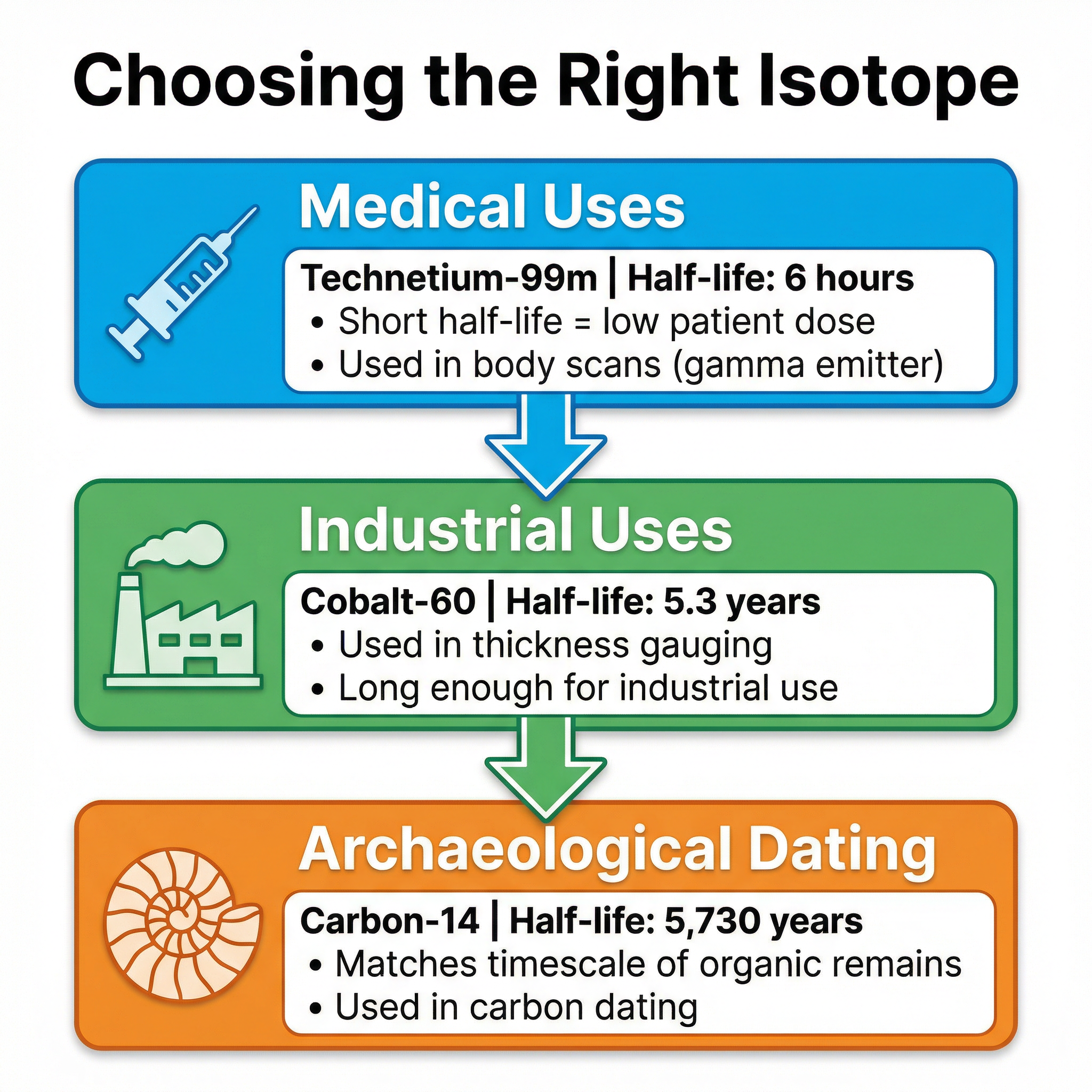
The choice of a radioactive isotope for a particular job is determined by its half-life and the type of radiation it emits. This is a very common context for AO2 and AO3 evaluation questions.
**Medical Tracers (e.g., Technetium-99m)**: Used to diagnose medical conditions. The isotope is injected into the patient and its movement around the body is tracked using a gamma camera.
- **Half-life**: Must be short (e.g., 6 hours for Tc-99m). This ensures the patient's exposure to radiation is minimised, as the source decays quickly. However, it must be long enough to allow the scan to be completed.
- **Radiation Type**: Must be a **gamma emitter**. Alpha and beta are too ionising and would be absorbed by body tissues, causing damage. Gamma radiation is weakly ionising and can pass out of the body to be detected.
**Industrial Thickness Gauging (e.g., Cobalt-60)**: Used to monitor the thickness of materials like paper or steel sheeting during production. A source is placed on one side and a detector on the other. If the thickness changes, the amount of radiation detected changes, and the machinery can be adjusted.
- **Half-life**: Must be long (e.g., 5.3 years for Co-60). This avoids the need for frequent replacement, which would be costly and impractical.
**Archaeological Dating (e.g., Carbon-14)**: Used to find the age of once-living materials. Living things absorb carbon, including a tiny proportion of radioactive Carbon-14. When they die, they stop absorbing carbon, and the C-14 decays with a half-life of 5,730 years. By measuring the remaining C-14 activity, scientists can estimate the age of the material.
- **Half-life**: Must be long enough to be relevant to the age of the artefact. A half-life of a few hours would be useless for dating a 10,000-year-old fossil.