AQA · A-Level · Geography
Course version: 7037 · Version from Sept 2018
Graphical skills: Dispersion diagrams.
Dispersion diagrams are one-dimensional graphs used to display the spread of a single variable, allowing geographers to visually assess data range, central tendency, and clustering.
Checked against the AQA 7037 specification (opens in a new tab) on .
- Point 7 of 7
- 4 key terms
Study notes
From the checked teaching notes for this specification point.
The idea
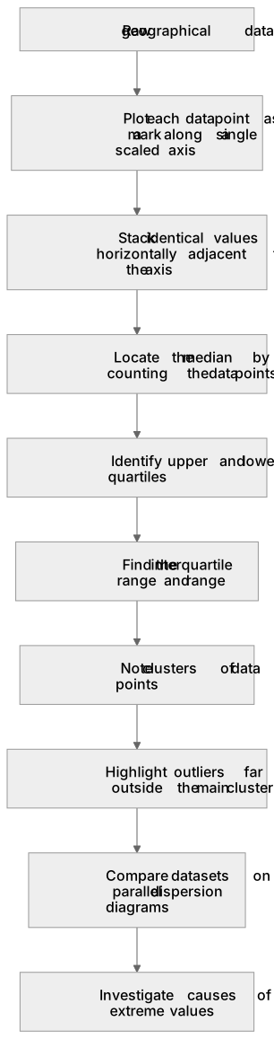
Dispersion diagrams are one-dimensional graphs used to display the spread of a single variable, allowing geographers to visually assess data range, central tendency, and clustering. Each data point is plotted as a mark along a single numerical axis. They are highly effective for comparing multiple datasets side-by-side, such as pebble sizes from two different beaches. By plotting data this way, students can easily locate the median, upper and lower quartiles, and the interquartile range to evaluate data reliability. Furthermore, dispersion diagrams clearly highlight anomalies or outliers that sit far outside the main cluster of data points, prompting further geographical investigation into the causes of these extreme values.
What earns the marks
- Construct a dispersion diagram by plotting individual data points accurately along a single scaled axis.
- Identify measures of central tendency (median) and spread (range, interquartile range) directly from the diagram.
- Compare the distribution, clustering, and spread of two or more datasets plotted on parallel dispersion diagrams.
- Identify and extract anomalous results (outliers) from the visual spread of the data points.
Common mistakes and how to put them right
Overlapping data points so that the total frequency of a specific value is obscured.
Put it right: Stack identical values horizontally adjacent to the axis so the frequency of that value is clearly visible.
Failing to use a consistent and appropriate scale for the axis, making comparison between different diagrams impossible.
Put it right: Ensure the axis covers the full range of all datasets being compared and uses consistent linear increments.
Confusing the median with the mean when interpreting the central tendency from the diagram.
Put it right: The diagram easily yields the median by counting the data points, whereas the mean requires calculation.
Exam tips
- When asked to compare two dispersion diagrams, explicitly mention differences in the median, range, and interquartile range using data from the axes.
- Look for clusters of data points; these indicate the most common values and are a key feature to describe in an exam answer.
- Always highlight any clear outliers in your analysis, as examiners often award marks for recognising anomalies.
Try the lesson
The start of the Graphical skills: Dispersion diagrams. lesson, made from checked teaching notes for this specification point.
Have a go first
A geographer plots individual pebble sizes from a beach along a single vertical axis, placing a dot for each measurement. What is the primary advantage of using this type of dispersion diagram rather than calculating a single mean value?
Listen
Dispersion diagrams are one-dimensional graphs used to display the spread of a single variable, allowing geographers to visually assess data range, central tendency, and clustering. Each data point is plotted as a mark along a single numerical axis. They are highly effective for comparing multiple datasets side-by-side, such as pebble sizes from two different beaches. By plotting data this way, students can easily locate the median, upper and lower quartiles, and the interquartile range to evaluate data reliability. Furthermore, dispersion diagrams clearly highlight anomalies or outliers that sit far outside the main cluster of data points, prompting further geographical investigation into the causes of these extreme values. A strong answer earns marks for these points. Construct a dispersion diagram by plotting individual data points accurately along a single scaled axis. Identify measures of central tendency (median) and spread (range, interquartile range) directly from the diagram. Compare the distribution, clustering, and spread of two or more datasets plotted on parallel dispersion diagrams. Identify and extract anomalous results (outliers) from the visual spread of the data points. A common slip: Overlapping data points so that the total frequency of a specific value is obscured. Instead, Stack identical values horizontally adjacent to the axis so the frequency of that value is clearly visible. Exam tip: When asked to compare two dispersion diagrams, explicitly mention differences in the median, range, and interquartile range using data from the axes.
See it
Key words
Say what each word means before you turn the card.
Dispersion diagrams
Try answering aloud or in your head before turning the card.
Outliers
Try answering aloud or in your head before turning the card.
Interquartile range
Try answering aloud or in your head before turning the card.
Median
Try answering aloud or in your head before turning the card.
See every definition
- Dispersion diagrams
- One-dimensional graphs used to display the spread of a single variable, with each data point plotted as a mark along a single numerical axis.
- Outliers
- Anomalies that sit far outside the main cluster of data points and prompt further geographical investigation into the causes of these extreme values.
- Interquartile range
- A measure of spread that can be located from the diagram to evaluate data reliability.
- Median
- A measure of central tendency that can easily be located from the diagram by counting the data points.
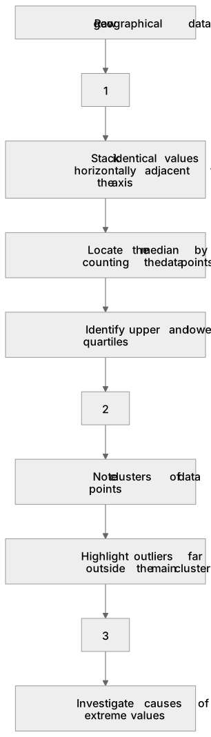
Label the diagram
Some boxes have lost their names. Pick the right name for each number.
1Box 1
2Box 2
3Box 3
There is more to this lesson
The full lesson goes on to check your understanding and help you earn the marks. Create a free account to carry on, with your progress saved.
A week of Premium from your first lesson · Then the free plan continues · No card, no charge
Test your understanding of Graphical skills: Dispersion diagrams.
Active recall beats re-reading. Take an instant quiz now to test what you’ve learned and lock it into long-term memory.
A week of Premium from your first lesson · Then the free plan continues · No card, no charge