Interpret diagrams for single-variable data, including understanding that…

The idea

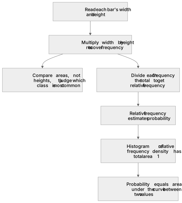
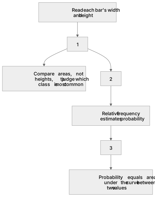
Single-variable diagrams summarise one measured variable. In a histogram, unequal class widths mean frequency is represented by the area of each bar, not its height. Frequency density is frequency divided by class width, so a bar of width 5 and height 4 represents a frequency of 20. To interpret such a diagram, read each bar's width and height, multiply them to recover frequency, and compare areas when judging which class is most common. This links directly to probability distributions: relative frequency, found by dividing each frequency by the total, estimates probability, and a histogram of relative frequency density has total area 1. Thus the same area principle underlies continuous probability density functions, where probability equals the area under the curve between two values.

What earns the marks

• States that in a histogram with unequal class widths, frequency equals frequency density multiplied by class width, so area represents frequency.
• Calculates a missing frequency by multiplying a bar's height by its class width, and a missing height by dividing frequency by class width.
• Compares classes correctly by area rather than by bar height when class widths differ.
• Explains that relative frequency estimates probability and that total relative frequency is 1.
• Links histogram area to probability density, where probability corresponds to area under a curve between two values.

Common mistakes and how to put them right

• Treating bar height as frequency when class widths are unequal.

  Put it right: Multiply height by width to obtain frequency.

• Forgetting to divide frequency by class width when drawing or completing a histogram.

  Put it right: Plot frequency density on the vertical axis.

• Assuming a histogram's total area equals the total frequency.

  Put it right: Total area equals total frequency only when frequency density is used, whereas relative frequency density gives total area 1.

Exam tips

• Label the vertical axis frequency density and show one area calculation to justify a frequency you read from a histogram.
• When asked to compare two classes, quote both areas and state the conclusion in the context of the data.
• Convert frequencies to relative frequencies before discussing probability, and check that they sum to 1.