Pearson Edexcel · A-Level · Mathematics
Course version: 9MA0 · Version from Mar 2026
Understand and use exponential growth and decay; use in modelling…
Full specification wording
Exponentials and logarithms: 6.7 Understand and use exponential growth and decay; use in modelling (examples may include the use of e in continuous compound interest, radioactive decay, drug concentration decay, exponential growth as a model for population growth); consideration of limitations and refinements of exponential models.
Exponential growth and decay describe quantities changing at a rate proportional to their current size, modelled by y = Ae^(kt) or y = Ab^t.
Checked against the Pearson Edexcel 9MA0 specification (opens in a new tab) on .
- Point 7 of 7
- 4 key terms
Study notes
From the checked teaching notes for this specification point.
The idea
Exponential growth and decay describe quantities changing at a rate proportional to their current size, modelled by y = Ae^(kt) or y = Ab^t. Growth occurs when k is positive, decay when k is negative. Continuous compound interest uses A = Pe^(rt), where P is the principal, r the annual rate and t the time in years. Radioactive decay uses N = N₀e^(−λt), with λ the decay constant and half-life t½ = ln 2 ÷ λ. Drug concentration often falls as C = C₀e^(−kt), and population growth may follow P = P₀e^(rt). Models assume constant rates and unlimited resources, so they have limitations: real populations face resource limits, drug clearance varies between patients, and decay rates may change. Refinements include logistic growth or piecewise models.
What earns the marks
- Sets up an exponential model of the form y = Ae^(kt) or y = Ab^t with parameters identified from the context.
- Interprets the sign of the rate constant: positive for growth, negative for decay.
- Uses the continuous compound interest formula A = Pe^(rt) correctly, keeping t in years and r as a decimal.
- Applies radioactive decay N = N₀e^(−λt) and links the decay constant to half-life using t½ = ln 2 ÷ λ.
- Models drug concentration decay or population growth with an appropriate exponential function and evaluates at a given time.
- Discusses limitations such as constant rate assumptions, resource limits or individual variation, and suggests a refinement such as a logistic model.
Common mistakes and how to put them right
Using a percentage rate directly as the exponent without converting to a decimal.
Put it right by writing r as a decimal, for example 5% as 0.05.
Treating a decay constant as positive in the exponent.
Put it right by using a negative exponent for decay.
Assuming exponential growth continues indefinitely.
Put it right by discussing resource limits and refinements such as logistic growth.
Exam tips
- Define each symbol and its units before substituting values into a model.
- Keep full calculator accuracy through intermediate steps and round only the final answer.
- When asked about limitations, link each limitation to a specific assumption of the model.
Try the lesson
The start of the Exponentials and logarithms: 6.7 Understand and use exponential growth and decay; use in modelling (examples may include the use of e in continuous compound interest, radioactive decay, drug concentration decay, exponential growth as a model for population growth); consideration of limitations and refinements of exponential models. lesson, made from checked teaching notes for this specification point.
Have a go first
A population of bacteria doubles every hour. Starting with 500 bacteria, how many are there after 3 hours?
Listen
Exponential growth and decay describe quantities changing at a rate proportional to their current size, modelled by y = Ae^(kt) or y = Ab^t. Growth occurs when k is positive, decay when k is negative. Continuous compound interest uses A = Pe^(rt), where P is the principal, r the annual rate and t the time in years. Radioactive decay uses N = N₀e^(−λt), with λ the decay constant and half-life t½ = ln 2 ÷ λ. Drug concentration often falls as C = C₀e^(−kt), and population growth may follow P = P₀e^(rt). Models assume constant rates and unlimited resources, so they have limitations: real populations face resource limits, drug clearance varies between patients, and decay rates may change. Refinements include logistic growth or piecewise models. A strong answer earns marks for these points. Sets up an exponential model of the form y = Ae^(kt) or y = Ab^t with parameters identified from the context. Interprets the sign of the rate constant: positive for growth, negative for decay. Uses the continuous compound interest formula A = Pe^(rt) correctly, keeping t in years and r as a decimal. Applies radioactive decay N = N₀e^(−λt) and links the decay constant to half-life using t½ = ln 2 ÷ λ. A common slip: Using a percentage rate directly as the exponent without converting to a decimal. Instead, writing r as a decimal, for example 5% as 0.05. Exam tip: Define each symbol and its units before substituting values into a model.
See it
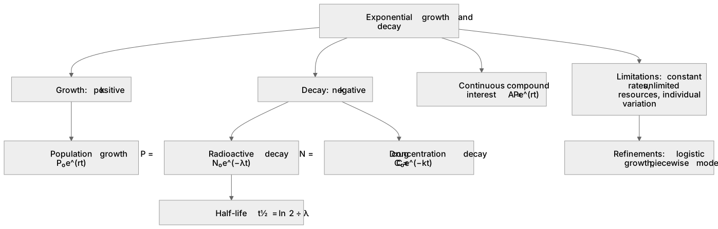
Key words
Say what each word means before you turn the card.
Exponential modelling
Try answering aloud or in your head before turning the card.
Continuous change
Try answering aloud or in your head before turning the card.
Half-life and decay constants
Try answering aloud or in your head before turning the card.
Model limitations and refinements
Try answering aloud or in your head before turning the card.
See every definition
- Exponential modelling
- Using exponential growth and decay functions, such as y = Ae^(kt) or y = Ab^t, to represent quantities changing at a rate proportional to their current size.
- Continuous change
- Change modelled using e, as in continuous compound interest A = Pe^(rt), where P is the principal, r the annual rate and t the time in years.
- Half-life and decay constants
- In radioactive decay N = N₀e^(−λt), λ is the decay constant and half-life is given by t½ = ln 2 ÷ λ.
- Model limitations and refinements
- Models assume constant rates and unlimited resources, so limitations include resource limits, varying drug clearance and changing decay rates; refinements include logistic growth or piecewise models.
Label the diagram
Some boxes have lost their names. Pick the right name for each number.
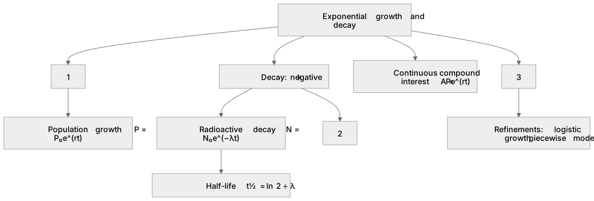
1Box 1
2Box 2
3Box 3
There is more to this lesson
The full lesson goes on to check your understanding and help you earn the marks. Create a free account to carry on, with your progress saved.
A week of Premium from your first lesson · Then the free plan continues · No card, no charge
Test your understanding of Exponentials and logarithms: 6.7 Understand and use exponential growth and decay; use in modelling (examples may include the use of e in continuous compound interest, radioactive decay, drug concentration decay, exponential growth as a model for population growth); consideration of limitations and refinements of exponential models.
Active recall beats re-reading. Take an instant quiz now to test what you’ve learned and lock it into long-term memory.
A week of Premium from your first lesson · Then the free plan continues · No card, no charge