Velocity-time graphs

Overview

Velocity-time graphs are a cornerstone of kinematics in GCSE Physics, providing a powerful visual method to describe and analyse an object's motion. For an examiner, these graphs are an excellent way to test a candidate's ability to apply mathematical skills in a physics context (AO2), interpret data, and make logical deductions. This topic, specification reference 1.7, requires you to master two key skills: calculating acceleration from the gradient of the graph, and determining the displacement (or distance travelled) by calculating the area underneath it. Questions often involve multi-stage journeys, requiring you to break down the graph into distinct sections of constant velocity, constant acceleration, and deceleration. Higher Tier candidates face the additional challenge of interpreting curved graphs, which represent non-uniform acceleration, and must be able to use a tangent to estimate instantaneous acceleration. A solid understanding here provides a crucial foundation for more advanced mechanics in A-Level Physics.

Key Concepts

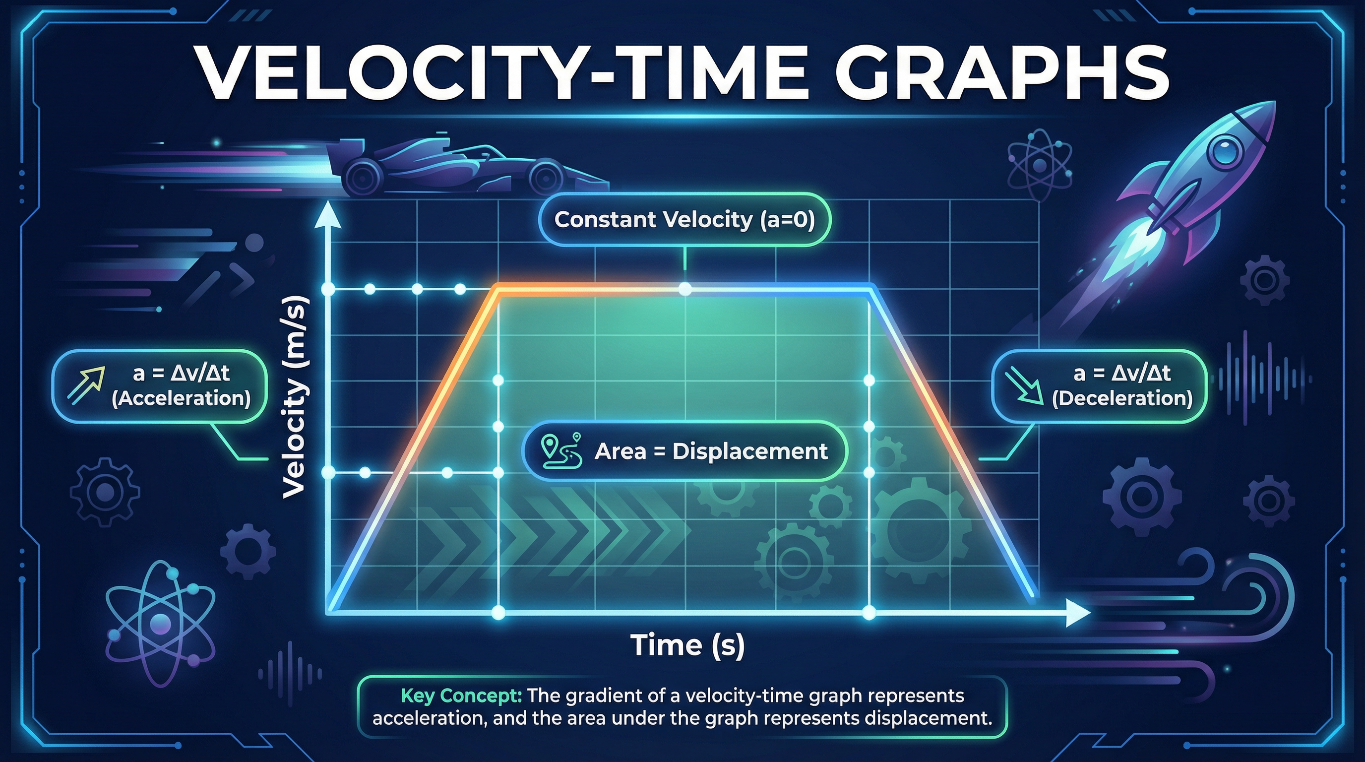
Concept 1: Interpreting the Axes and Gradient

A velocity-time graph plots the velocity of an object on the vertical (y) axis against time on the horizontal (x) axis. The single most important skill is to understand that the gradient (steepness) of the line represents acceleration. A steeper line means a greater acceleration. A positive gradient indicates acceleration, a negative gradient indicates deceleration, and a zero gradient (a flat, horizontal line) means the acceleration is zero, which signifies constant velocity. This is the most common point of confusion; candidates frequently mistake a horizontal line for 'stationary'. An object is only stationary if the line is on the x-axis itself (where velocity = 0 m/s).

Example: If a line goes from (2s, 5m/s) to (7s, 20m/s), the gradient is the change in velocity (20 - 5 = 15 m/s) divided by the change in time (7 - 2 = 5 s). The acceleration is 15 / 5 = 3 m/s².

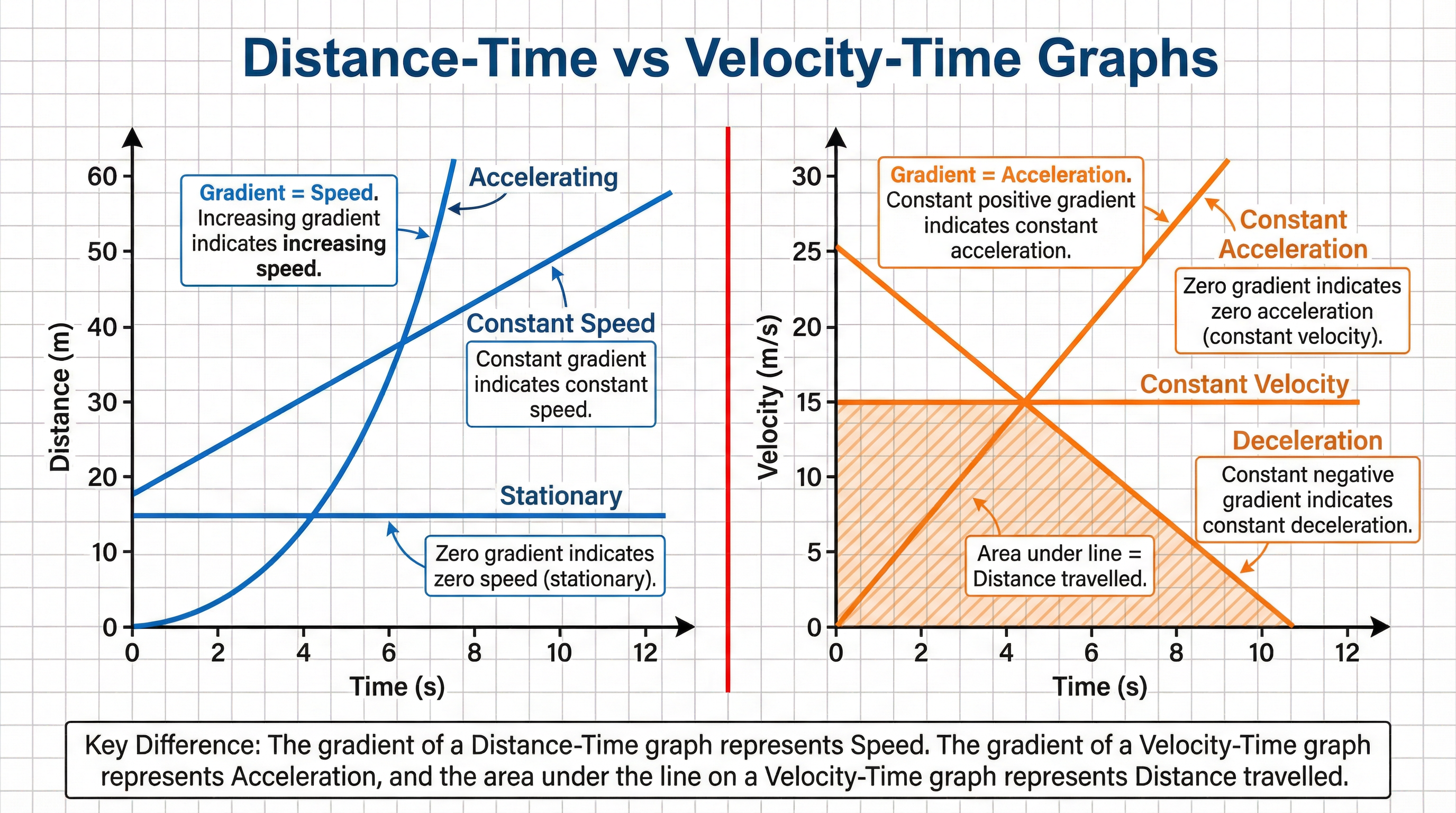
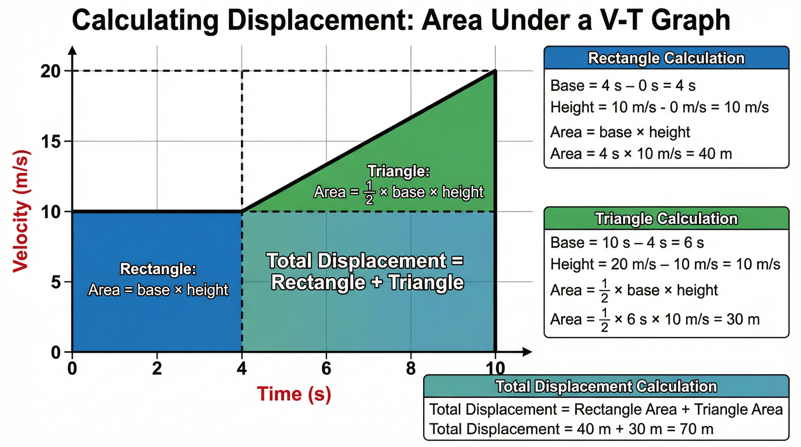
Concept 2: Calculating Displacement from Area

The second core skill is understanding that the area under the line on a velocity-time graph represents the displacement of the object (how far it has moved from its starting point). To find the total displacement for a journey, you must calculate the total area between the graph line and the x-axis. For any journey involving changes in acceleration, this often means the area is a composite shape. Candidates are expected to divide this area into simpler, standard geometric shapes—rectangles and triangles—to calculate the area of each part and then sum them. Credit is given for clearly showing how the area has been split.

Example: An object travels at a constant velocity of 10 m/s for 4 seconds. The area is a rectangle: Area = 10 m/s * 4 s = 40 m. If it then accelerates for 6 seconds, forming a triangle on top of the rectangle, you must calculate the area of that triangle (Area = ½ * base * height) and add it to the rectangle's area.

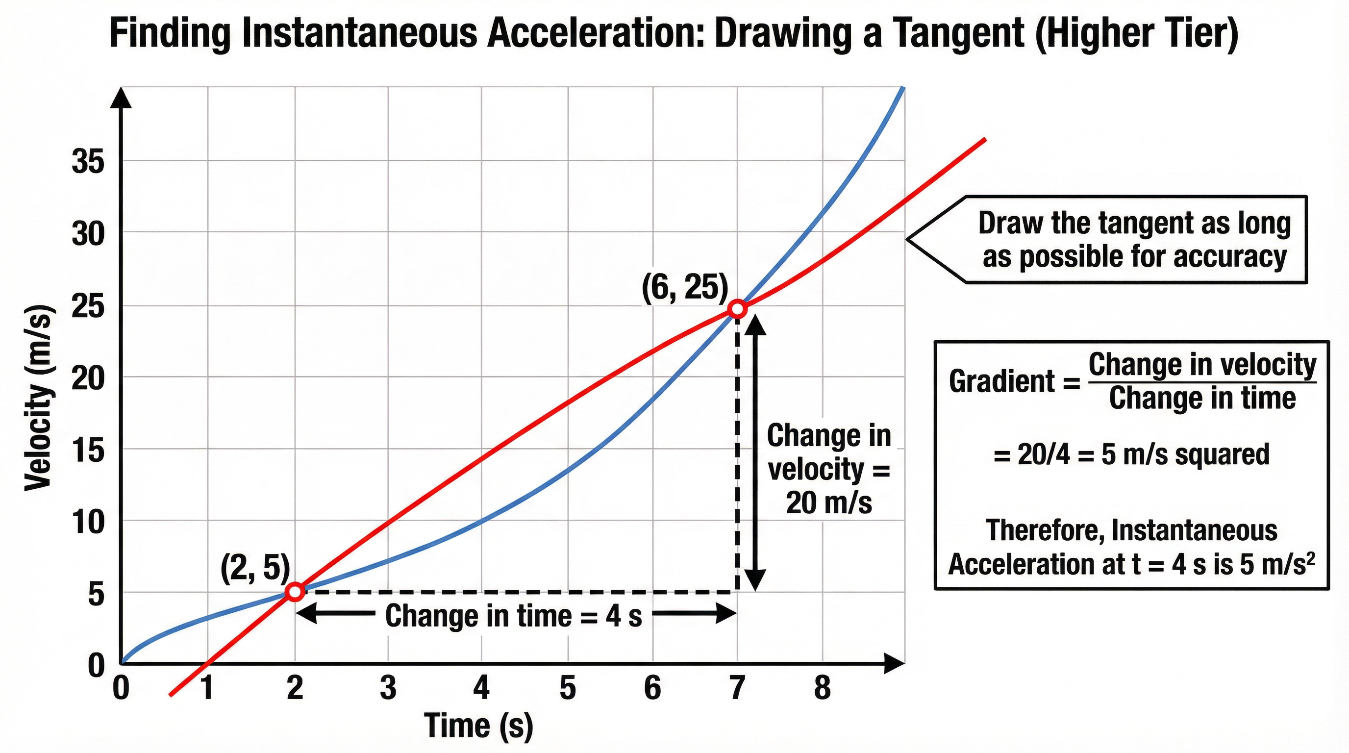
Concept 3: Non-Uniform Acceleration (Higher Tier Only)

For Higher Tier candidates, the graph may not consist of straight lines. A curved line indicates that the acceleration is changing (it is non-uniform). You cannot calculate a single gradient for a curve. Instead, examiners will ask for the instantaneous acceleration at a specific point in time. To find this, you must draw a tangent to the curve at that exact point. A tangent is a straight line that just touches the curve at that point without crossing it. The gradient of this tangent is equal to the instantaneous acceleration at that moment. Marks are awarded for drawing a sufficiently long and accurate tangent and then correctly calculating its gradient.

Example: To find the acceleration at t = 4s on a curved graph, you would place a ruler on the graph, touching the curve at t=4s, and draw a straight line. You would then pick two points on this tangent line (as far apart as possible) and calculate the gradient as normal.

Mathematical/Scientific Relationships

• Acceleration (from gradient): Must memorise.
  a = (v - u) / t or a = Δv / Δt
  Where: a = acceleration (m/s²), v = final velocity (m/s), u = initial velocity (m/s), t = time taken (s), Δv = change in velocity.

• Displacement (from area of a rectangle): Must memorise.
  Area = base × height (for constant velocity sections)

• Displacement (from area of a triangle): Must memorise.
  Area = ½ × base × height (for sections of constant acceleration/deceleration from rest or to rest).

• Displacement (from area of a trapezium): Given on formula sheet, but often easier to split into a rectangle and triangle.
  Area = ½(a+b)h where a and b are the parallel sides (the initial and final velocities) and h is the width (the time interval).

Practical Applications

While there isn't a specific required practical for velocity-time graphs, the principles are fundamental to analysing motion in all dynamics experiments. For example, if you were investigating the motion of a trolley rolling down a ramp, you could use a motion sensor connected to a data logger to plot a real-time velocity-time graph. The graph would likely be a straight line through the origin, showing constant acceleration due to gravity. You could then calculate the gradient to find the experimental value for the trolley's acceleration. This links directly to investigations of Newton's Second Law (F=ma).