Pearson Edexcel · A-Level · Mathematics
Course version: 9MA0 · Version from Mar 2026
Understand and use numerical integration of functions, including the use…
Full specification wording
Numerical methods: 9.4 Understand and use numerical integration of functions, including the use of the trapezium rule and estimating the approximate area under a curve and limits that it must lie between.
Numerical integration estimates a definite integral when an antiderivative is unavailable or inconvenient.
Checked against the Pearson Edexcel 9MA0 specification (opens in a new tab) on .
- Point 4 of 5
- 4 key terms
Study notes
From the checked teaching notes for this specification point.
The idea
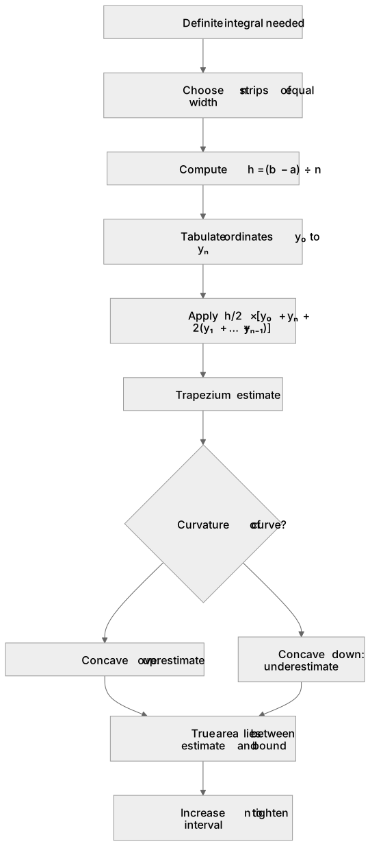
Numerical integration estimates a definite integral when an antiderivative is unavailable or inconvenient. The trapezium rule replaces the area under y = f(x) between x = a and x = b with n strips of equal width h = (b − a) ÷ n. Each strip is a trapezium, so the total is h/2 × [y₀ + yₙ + 2(y₁ + y₂ + … + yₙ₋₁)]. For example, with h = 0.5, y₀ = 1, y₁ = 2, y₂ = 5, the estimate is 0.5/2 × [1 + 5 + 2(2)] = 2.5. A curve that is concave up lies below its chords, so the rule overestimates; concave down gives an underestimate. The true area therefore lies between the trapezium estimate and a bound obtained by considering the curve's curvature, and increasing n generally tightens that interval.
What earns the marks
- States the trapezium rule correctly as h/2 × [y₀ + yₙ + 2(y₁ + y₂ + … + yₙ₋₁)] with h = (b − a) ÷ n and uses it to estimate a definite integral.
- Computes strip width h accurately from the limits and number of strips, then tabulates ordinates y₀ to yₙ at x = a, a + h, …, b, showing sufficient working.
- Explains that the estimate is approximate because straight chords replace the curve, and links the direction of error to whether the curve is concave up or concave down over the interval.
- Determines limits between which the true area must lie, for example by comparing the trapezium estimate with an inscribed or circumscribed bound, and interprets the result in context.
- Uses increased n or decreased h to improve the estimate and comments on convergence towards the true area, recognising that the rule is exact for linear functions.
Common mistakes and how to put them right
Doubling the first and last ordinates instead of only the interior ordinates.
Put it right by applying the factor 2 solely to y₁ through yₙ₋₁.
Using h = b − a rather than h = (b − a) ÷ n.
Put it right by dividing the interval width by the number of strips before substituting.
Assuming the trapezium rule always underestimates.
Put it right by checking concavity, since concave-up curves give overestimates and concave-down curves give underestimates.
Exam tips
- Write down h, the ordinate values and the bracket sum separately before evaluating, so arithmetic slips are easy to spot and method is visible.
- When asked for limits, give a lower and an upper value with a brief justification based on curvature rather than quoting the estimate alone.
- Check whether the question specifies the number of ordinates or strips; if ordinates are given, n is one less than the number of ordinates.
Try the lesson
The start of the Numerical methods: 9.4 Understand and use numerical integration of functions, including the use of the trapezium rule and estimating the approximate area under a curve and limits that it must lie between. lesson, made from checked teaching notes for this specification point.
Have a go first
The trapezium rule is used with two strips of equal width to estimate the area under the curve y = x² between x = 0 and x = 2. What is the value of this estimate?
Listen
Numerical integration estimates a definite integral when an antiderivative is unavailable or inconvenient. The trapezium rule replaces the area under y = f(x) between x = a and x = b with n strips of equal width h = (b − a) ÷ n. Each strip is a trapezium, so the total is h/2 × [y₀ + yₙ + 2(y₁ + y₂ + … + yₙ₋₁)]. For example, with h = 0.5, y₀ = 1, y₁ = 2, y₂ = 5, the estimate is 0.5/2 × [1 + 5 + 2(2)] = 2.5. A curve that is concave up lies below its chords, so the rule overestimates; concave down gives an underestimate. The true area therefore lies between the trapezium estimate and a bound obtained by considering the curve's curvature, and increasing n generally tightens that interval. A strong answer earns marks for these points. States the trapezium rule correctly as h/2 × [y₀ + yₙ + 2(y₁ + y₂ + … + yₙ₋₁)] with h = (b − a) ÷ n and uses it to estimate a definite integral. Computes strip width h accurately from the limits and number of strips, then tabulates ordinates y₀ to yₙ at x = a, a + h, …, b, showing sufficient working. Explains that the estimate is approximate because straight chords replace the curve, and links the direction of error to whether the curve is concave up or concave down over the interval. Determines limits between which the true area must lie, for example by comparing the trapezium estimate with an inscribed or circumscribed bound, and interprets the result in context. A common slip: Doubling the first and last ordinates instead of only the interior ordinates. Instead, applying the factor 2 solely to y₁ through yₙ₋₁. Exam tip: Write down h, the ordinate values and the bracket sum separately before evaluating, so arithmetic slips are easy to spot and method is visible.
See it
Key words
Say what each word means before you turn the card.
Trapezium rule
Try answering aloud or in your head before turning the card.
Strip width
Try answering aloud or in your head before turning the card.
Concave up
Try answering aloud or in your head before turning the card.
Concave down
Try answering aloud or in your head before turning the card.
See every definition
- Trapezium rule
- Replaces the area under y = f(x) between x = a and x = b with n strips of equal width, each strip being a trapezium.
- Strip width
- Equal width h = (b − a) ÷ n, dividing the interval width by the number of strips.
- Concave up
- A curve that lies below its chords, so the rule overestimates the true area.
- Concave down
- A curve that gives an underestimate of the true area under the rule.
Label the diagram
Some boxes have lost their names. Pick the right name for each number.
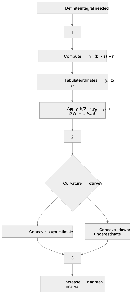
1Box 1
2Box 2
3Box 3
There is more to this lesson
The full lesson goes on to check your understanding and help you earn the marks. Create a free account to carry on, with your progress saved.
A week of Premium from your first lesson · Then the free plan continues · No card, no charge
Test your understanding of Numerical methods: 9.4 Understand and use numerical integration of functions, including the use of the trapezium rule and estimating the approximate area under a curve and limits that it must lie between.
Active recall beats re-reading. Take an instant quiz now to test what you’ve learned and lock it into long-term memory.
A week of Premium from your first lesson · Then the free plan continues · No card, no charge