Efficiency and Complexity — OCR GCSE Study Guide
Exam Board: OCR | Level: GCSE
Unlock top marks in OCR GCSE Computer Science by mastering algorithm efficiency and complexity. This guide breaks down how to compare algorithms like an examiner, using Big O notation to analyse speed and scalability, ensuring you can justify why one search or sort is better than another.
## Overview
Welcome to Topic 6.5: Efficiency and Complexity. In computer science, it's not enough to just write code that works; it must also be efficient. This topic explores how we measure and compare the performance of algorithms, a crucial skill for any programmer. We analyse how an algorithm's execution time and memory usage scale as the input data grows. Understanding this allows us to select the best algorithm for a given task, especially when dealing with large datasets where efficiency is paramount. For your exam, expect questions that require you to compare the efficiency of different search and sort algorithms, often using Big O notation. You will need to justify your choices, linking them to concepts like time complexity and space complexity, which are fundamental to building robust and scalable software.
{{asset:efficiency_and_complexity_podcast.mp3}}
## Key Concepts
### Concept 1: Computational Complexity
Computational complexity is the measure of the resources (time and space) an algorithm consumes as the size of the input increases. **Time complexity** refers to the amount of time an algorithm takes to complete, while **space complexity** refers to the amount of memory (RAM) it requires. In your exam, time complexity is the more frequently tested concept. We use a formal system called **Big O notation** to classify algorithms based on how their resource usage grows. This provides a high-level understanding of their performance, allowing us to compare them in a standardised way.
**Example**: An algorithm that checks every item in a list of size 'n' has a time complexity that grows linearly with 'n'. If the list doubles, the time taken roughly doubles. An algorithm that instantly finds an item regardless of list size has a constant time complexity.
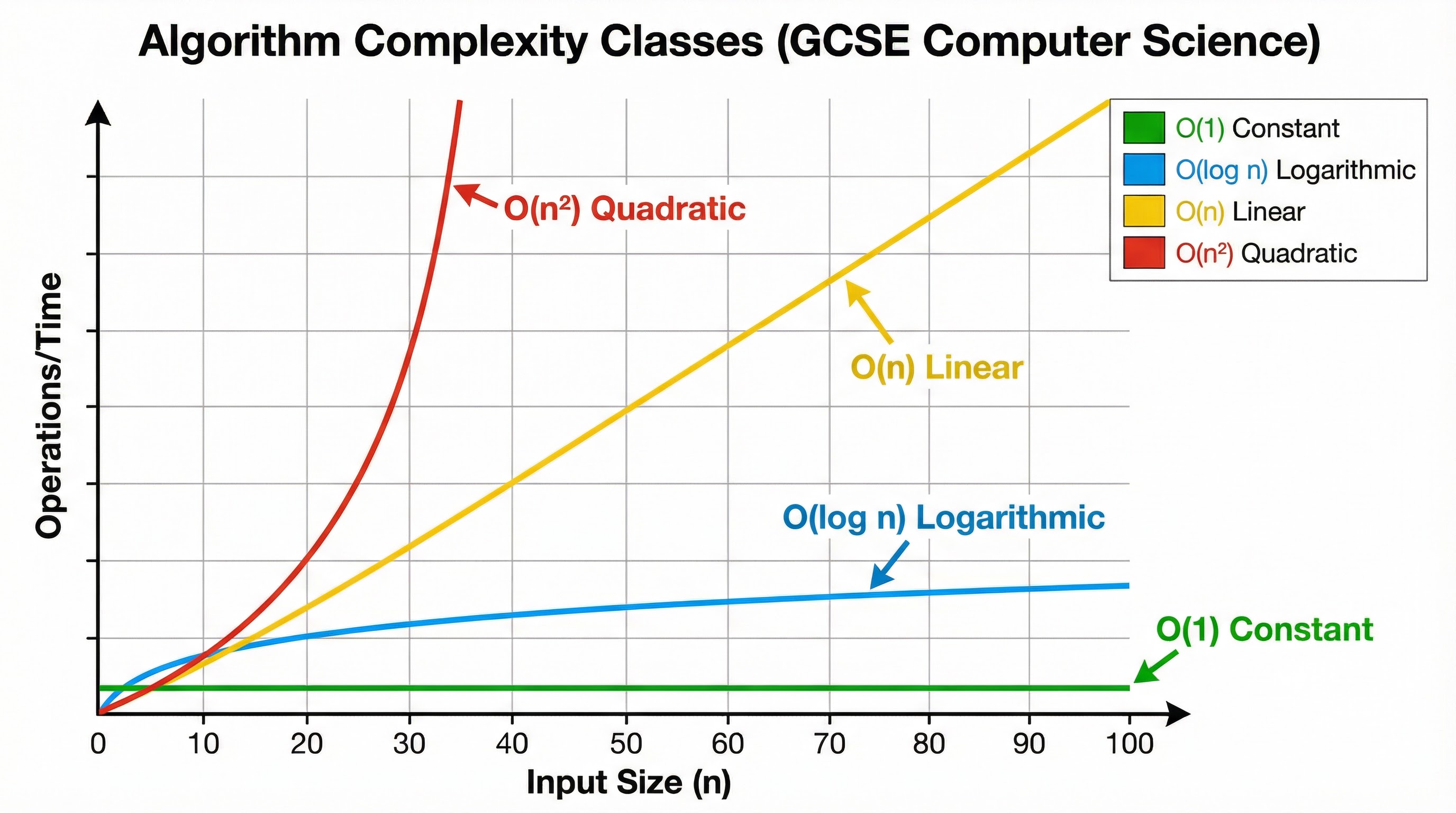
### Concept 2: Big O Notation
Big O notation is the standard way to express an algorithm's efficiency. It describes the worst-case scenario, giving an upper bound on how the execution time or memory usage will grow. For GCSE, you need to be familiar with the following classes:
* **O(1) - Constant Time**: The algorithm takes the same amount of time regardless of the input size. This is the most efficient complexity class.
* **Example**: Accessing an element in an array using its index.
* **O(log n) - Logarithmic Time**: The time taken increases very slowly as the input size grows. The algorithm becomes more efficient per item as the dataset gets larger.
* **Example**: Binary search.
* **O(n) - Linear Time**: The time taken is directly proportional to the input size. If the input size doubles, the time taken doubles.
* **Example**: Linear search.
* **O(n²) - Quadratic Time**: The time taken is proportional to the square of the input size. This is inefficient for large datasets.
* **Example**: Bubble sort.
### Concept 3: Search Algorithms
Searching is a fundamental operation. You need to know two key algorithms:
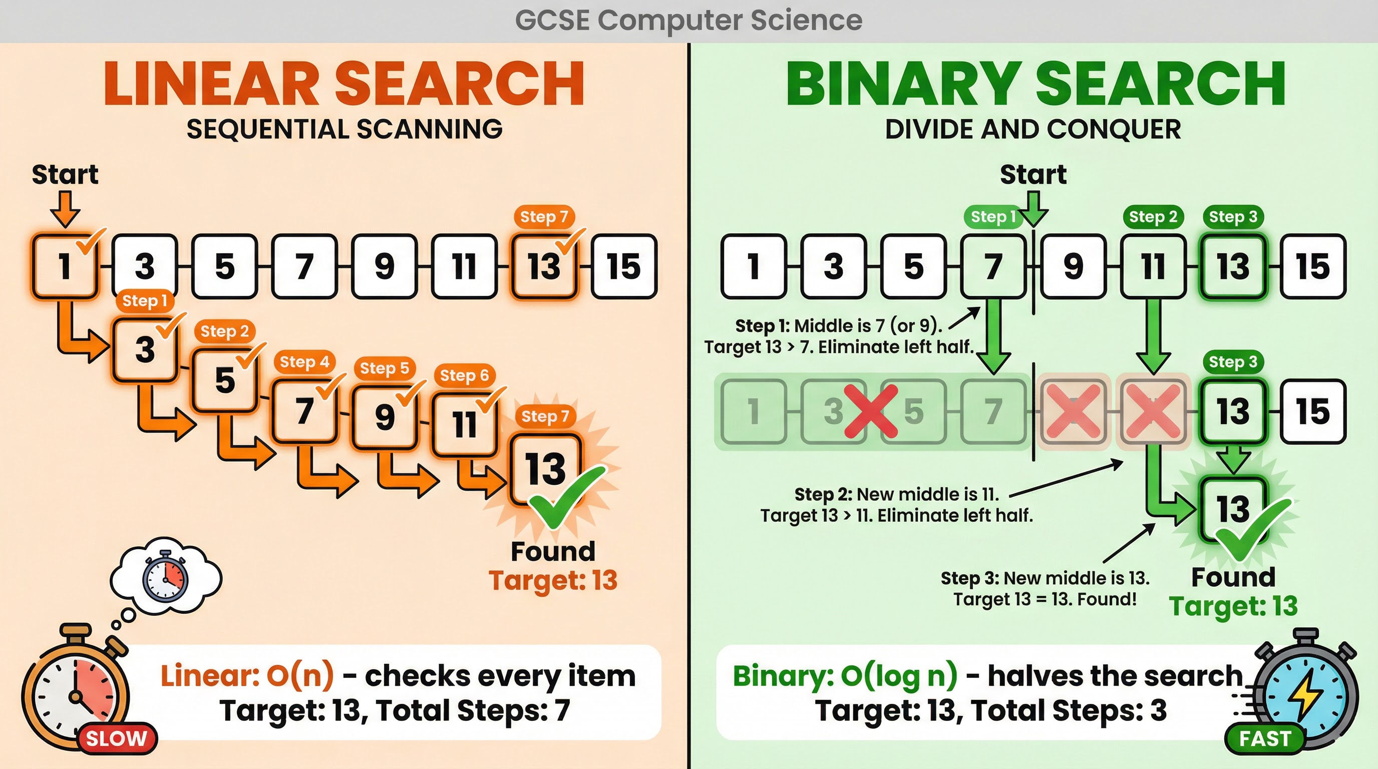
* **Linear Search**: This algorithm sequentially checks each element in a list until the target value is found or the end of the list is reached. It is simple to implement and can be used on any list, sorted or unsorted. Its time complexity is **O(n)**.
* **Binary Search**: This is a much more efficient 'divide and conquer' algorithm, but it **requires the list to be sorted**. It works by repeatedly dividing the search interval in half. It compares the target value to the middle element; if they are not equal, the half in which the target cannot lie is eliminated, and the search continues on the remaining half. Its time complexity is **O(log n)**.
### Concept 4: Sorting Algorithms
Sorting arranges items in a specific order. You need to understand the mechanics and efficiency of these algorithms:
* **Bubble Sort**: This simple algorithm repeatedly steps through the list, compares adjacent elements, and swaps them if they are in the wrong order. The passes through the list are repeated until the list is sorted. It is very inefficient for large lists, with a time complexity of **O(n²)**.
* **Merge Sort**: A more efficient 'divide and conquer' algorithm. It works by recursively splitting the list into halves until each sub-list contains a single element. Then, it merges the sub-lists back together in a sorted manner. Its time complexity is **O(n log n)**, making it much faster than bubble sort for large datasets.
* **Insertion Sort**: This algorithm builds the final sorted list one item at a time. It iterates through the input elements and inserts each element into its correct position in the sorted part of the list. It is efficient for small datasets or mostly sorted lists, with a worst-case time complexity of **O(n²)**.
## Mathematical/Scientific Relationships
Big O notation is the key mathematical relationship in this topic. It describes the growth rate of functions. While the underlying mathematics can be complex, for GCSE you only need to understand the relative performance of the key complexity classes.
| Big O Notation | Name | Performance Ranking | Must Memorise |
|----------------|---------------|---------------------|--------------------|
| O(1) | Constant | 1 (Fastest) | Must memorise |
| O(log n) | Logarithmic | 2 | Must memorise |
| O(n) | Linear | 3 | Must memorise |
| O(n log n) | Linearithmic | 4 | Must memorise |
| O(n²) | Quadratic | 5 (Slowest) | Must memorise |
## Practical Applications
* **Databases**: When you search for a product on Amazon, efficient search algorithms are used to quickly find relevant items from millions of products. Databases often use highly optimised search and sort algorithms (like variants of B-Trees, which are related to binary search) to handle massive amounts of data.
* **Social Media**: When your social media feed is generated, algorithms sort content based on relevance, recency, and your past interactions. The efficiency of these sorting algorithms directly impacts how quickly your feed loads.
* **GPS Navigation**: Route-finding apps like Google Maps use complex graph algorithms (like Dijkstra's algorithm) to find the shortest path. The efficiency of these algorithms is critical for providing real-time directions.