Graphs

Overview

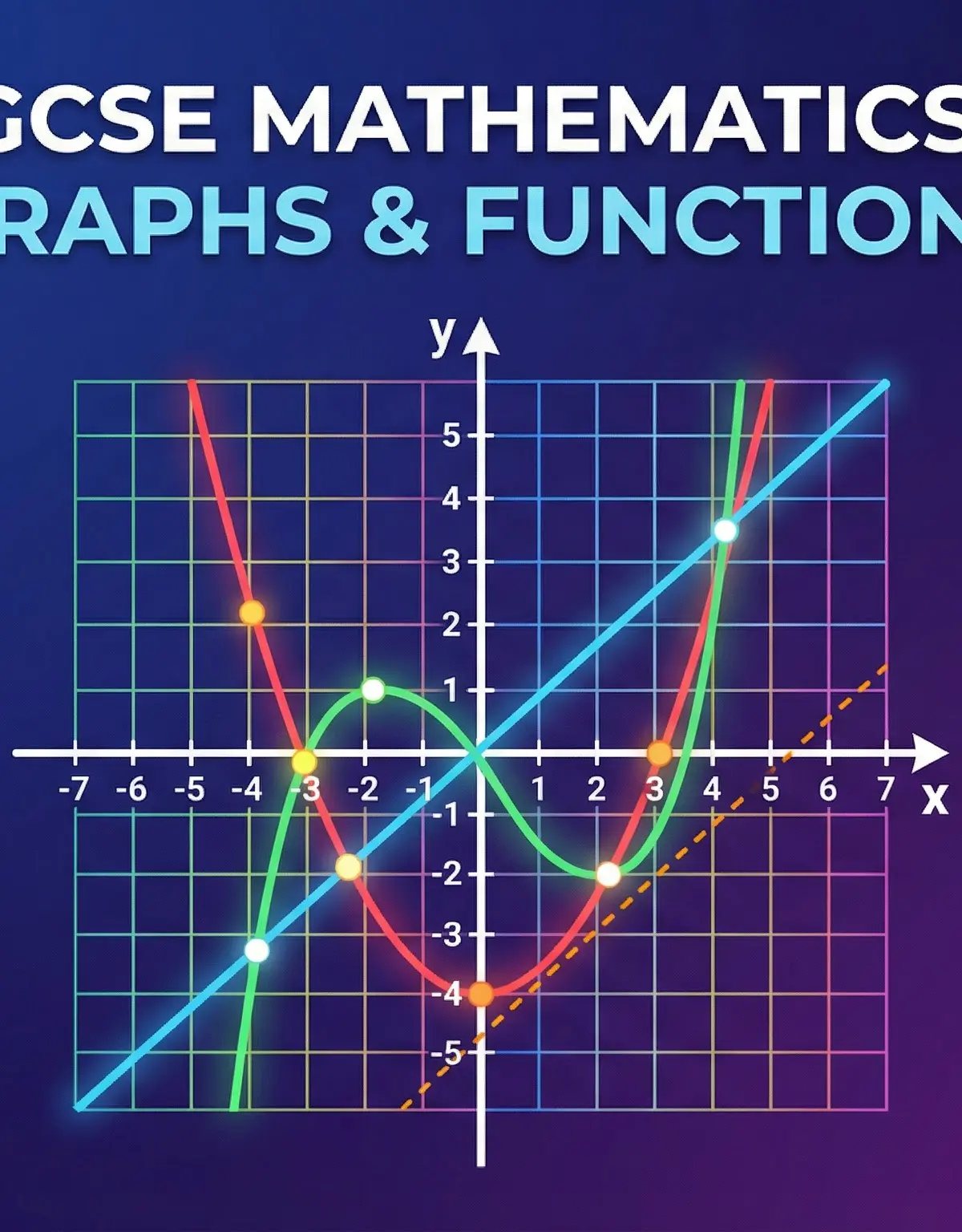
Welcome to the study of Graphs for OCR GCSE Mathematics (2.4). This topic is a cornerstone of the mathematics curriculum, forming the bridge between abstract algebra and visual geometry. For many candidates, mastering graphs is the key to unlocking higher grades, as it tests your fluency in plotting functions, interpreting real-world scenarios, and applying precise analytical techniques. Examiners frequently use graph-based questions to assess a wide range of skills, from fundamental plotting (AO1) to problem-solving in context (AO3). A solid understanding of how an equation like y = mx + c translates into a visual line is not just a skill; it's a new way of seeing mathematics. This guide will equip you with the core knowledge and, crucially, the exam techniques required to turn graph questions into a reliable source of marks.

Key Concepts

Concept 1: The Anatomy of a Linear Graph

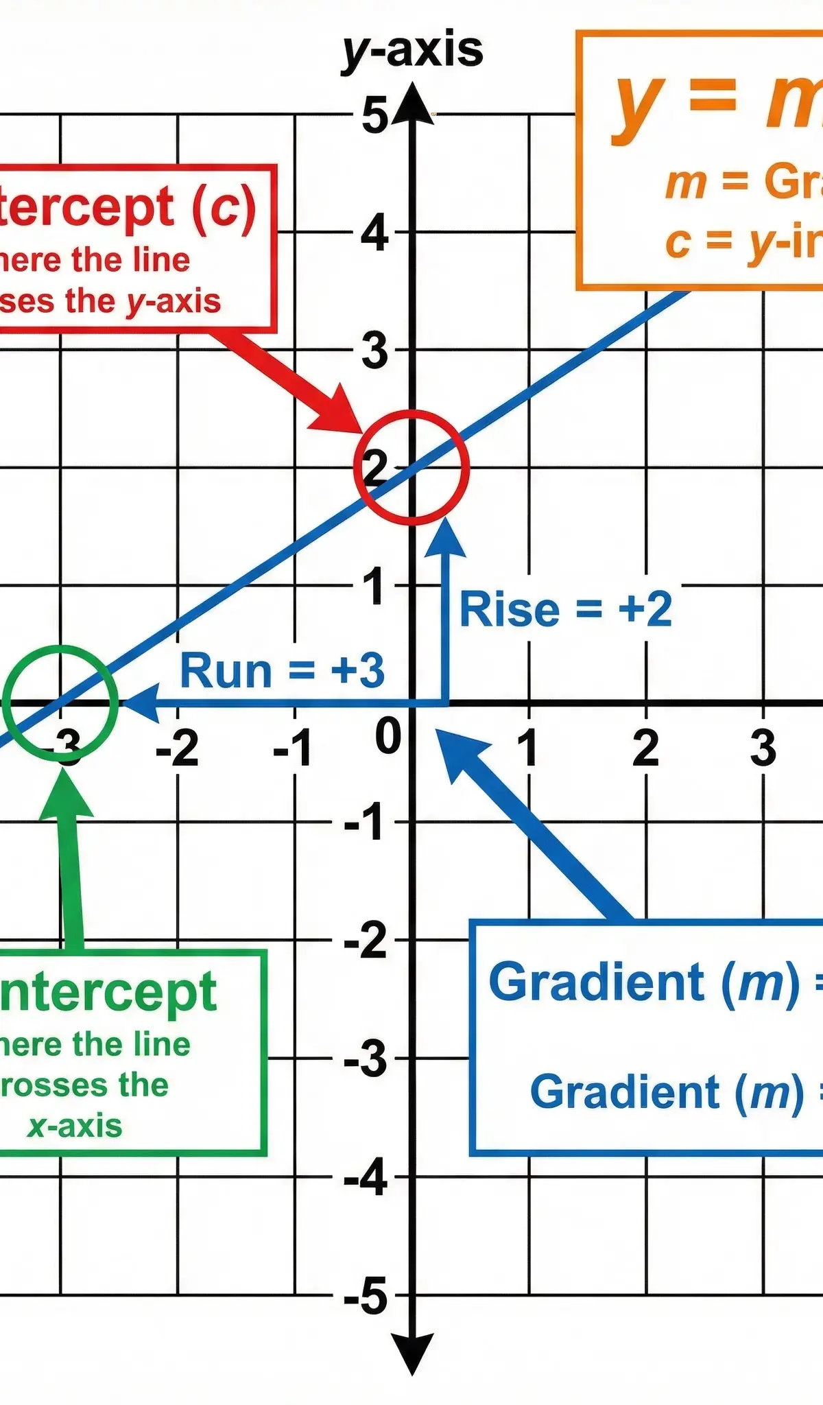
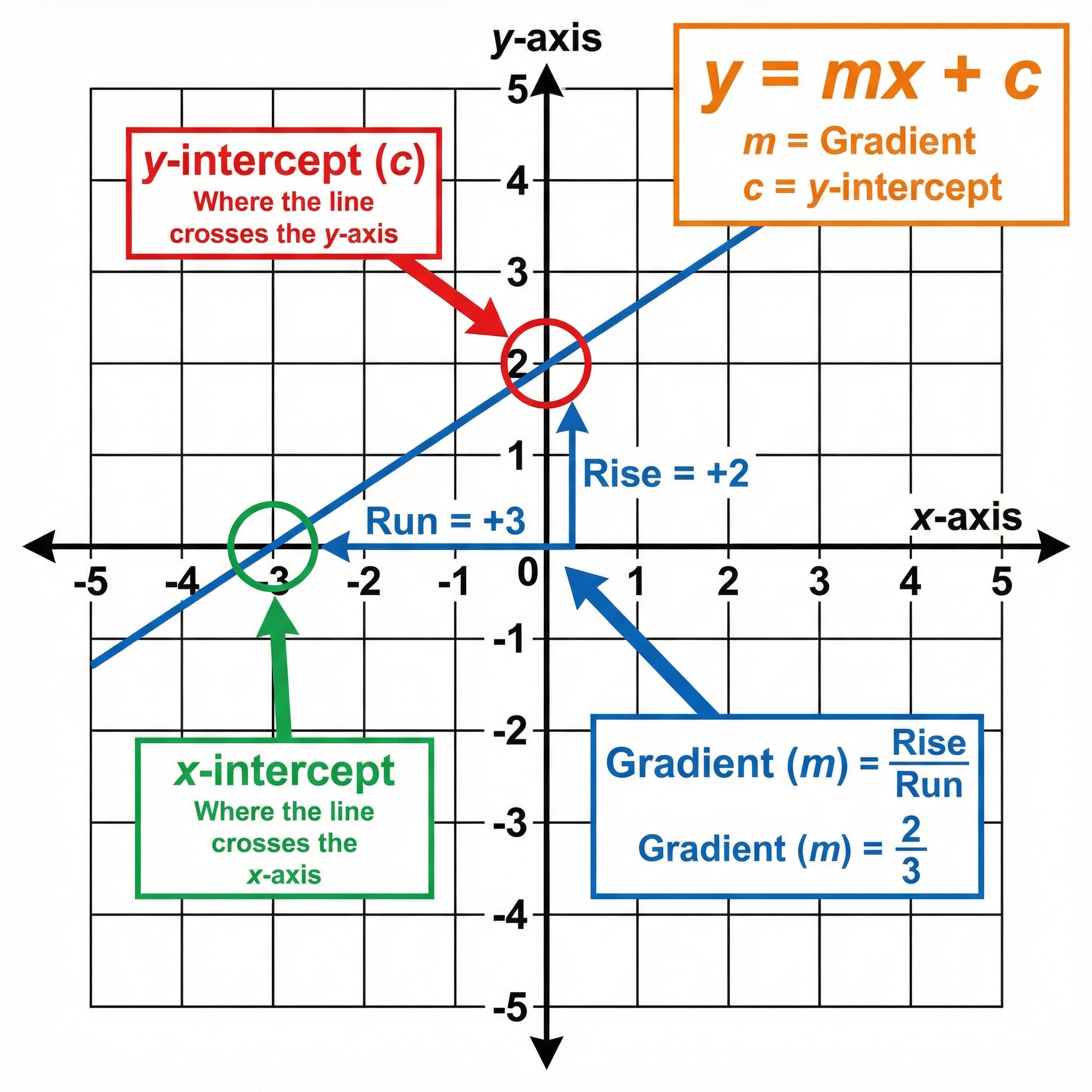
A linear graph is the simplest form of graphical representation, always forming a straight line. Its behaviour is entirely defined by the equation y = mx + c. Understanding what each part of this equation does is critical for earning marks.

• m is the Gradient: This value tells you how steep the line is. A positive gradient means the line slopes upwards from left to right. A negative gradient means it slopes downwards. The larger the number (positive or negative), the steeper the line. You calculate it using the formula: Gradient = (Change in y) / (Change in x), often remembered as 'rise over run'.
• c is the y-intercept: This is the point where the line physically crosses the vertical y-axis. In the equation, it's the constant term. If an equation is y = 2x + 5, the line will cross the y-axis at the point (0, 5). Credit is given by examiners for correctly identifying this point.

Concept 2: Mastering Quadratic Graphs

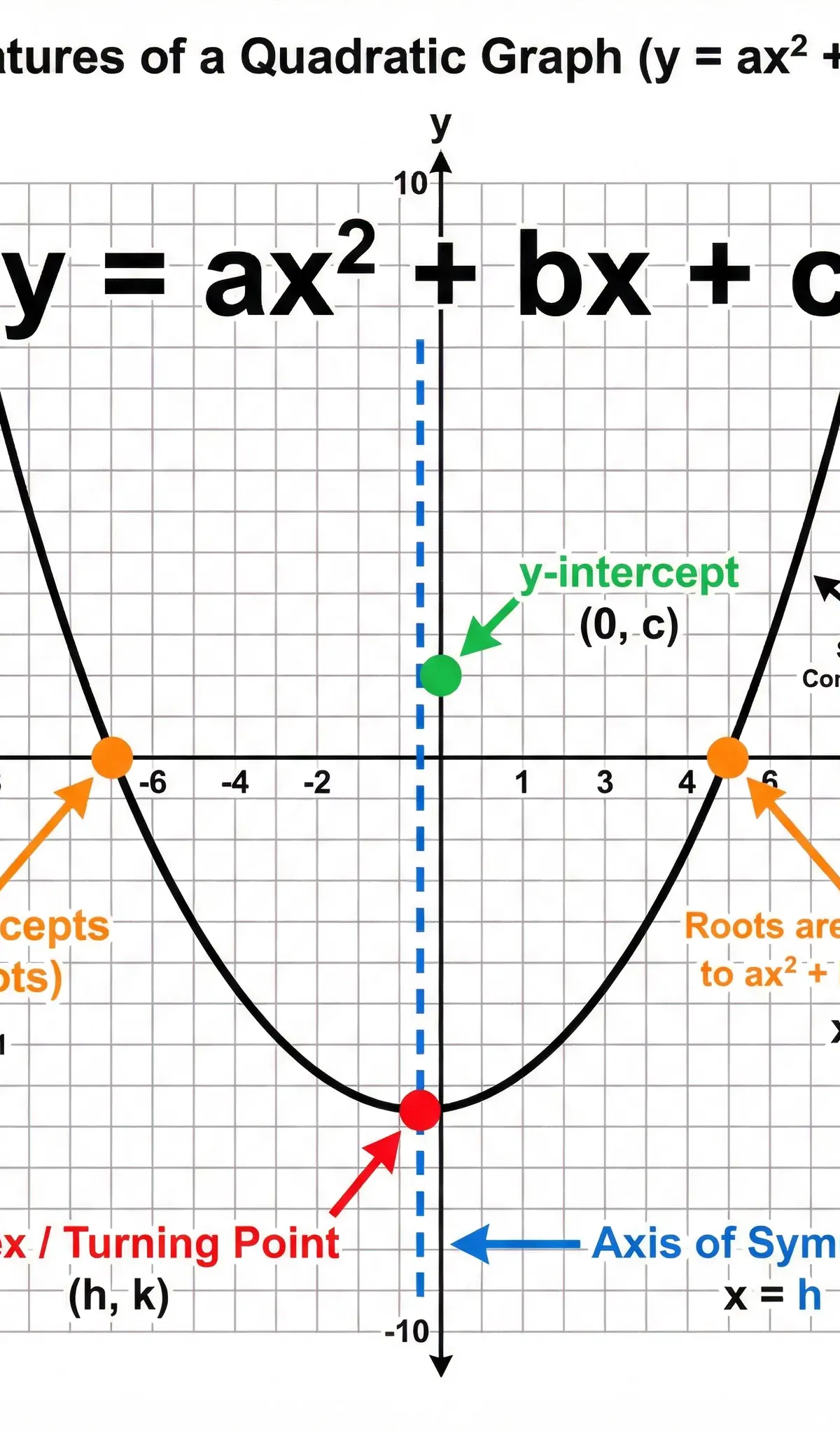
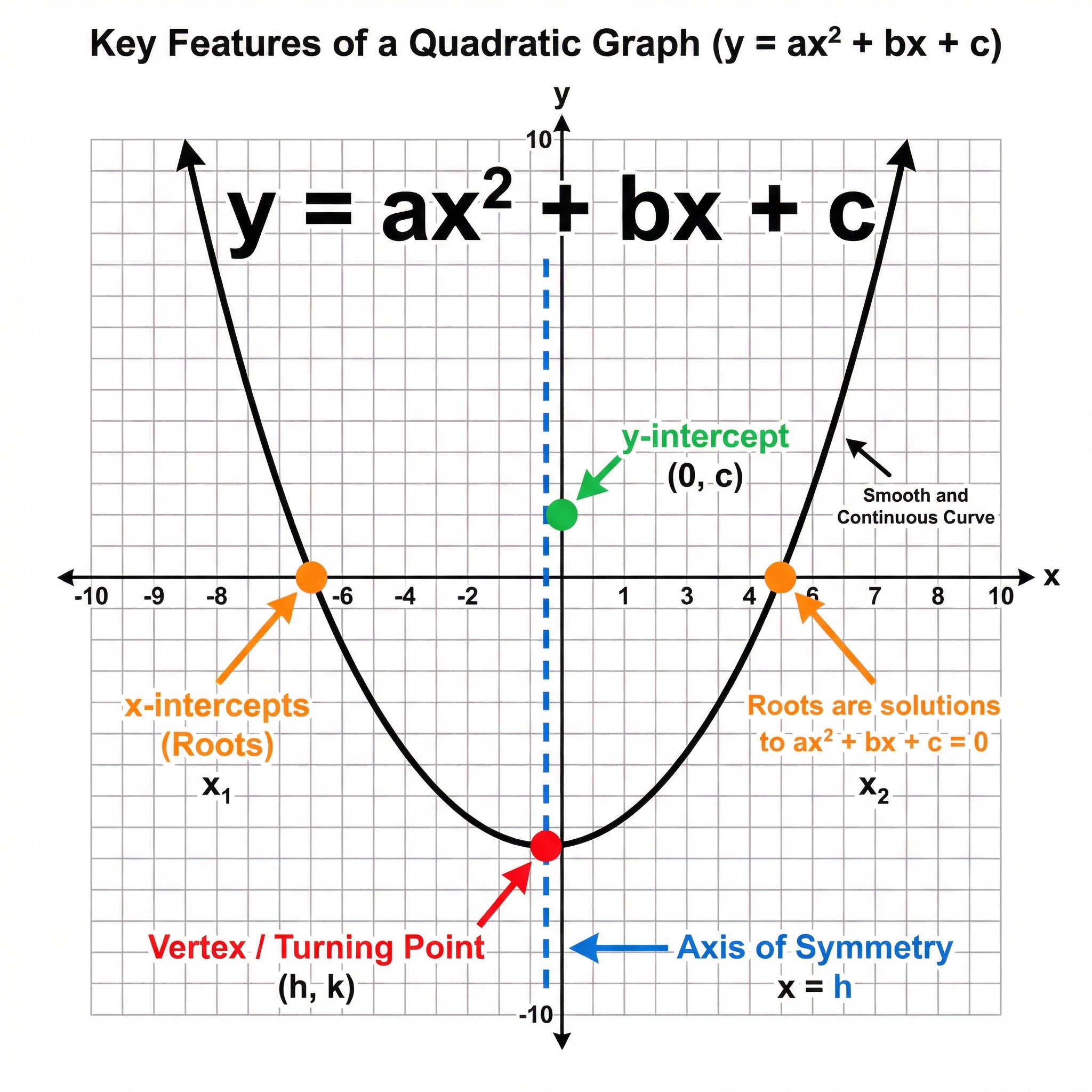
Quadratic graphs produce a smooth, symmetrical curve called a parabola. Their equation includes an x² term, with the general form being y = ax² + bx + c. Unlike linear graphs, their gradient is constantly changing.

• Shape: If the a value (the coefficient of x²) is positive, the parabola is U-shaped. If a is negative, it's an upside-down U-shape.
• Key Features: To earn full marks, you must identify and label:
  • Vertex (Turning Point): The minimum or maximum point of the curve.
  • Roots (x-intercepts): The points where the curve crosses the x-axis. These are the solutions to the equation ax² + bx + c = 0.
  • y-intercept: The point where the curve crosses the y-axis, which is always at (0, c).
  • Axis of Symmetry: A vertical line that cuts the parabola into two mirror images. Its equation is x = k, where k is the x-coordinate of the vertex.

Examiners award a specific mark (B1) for drawing a smooth, continuous curve through all plotted points. Using a ruler to join the dots is a guaranteed way to lose this mark.

Concept 3: Calculating and Interpreting Gradient

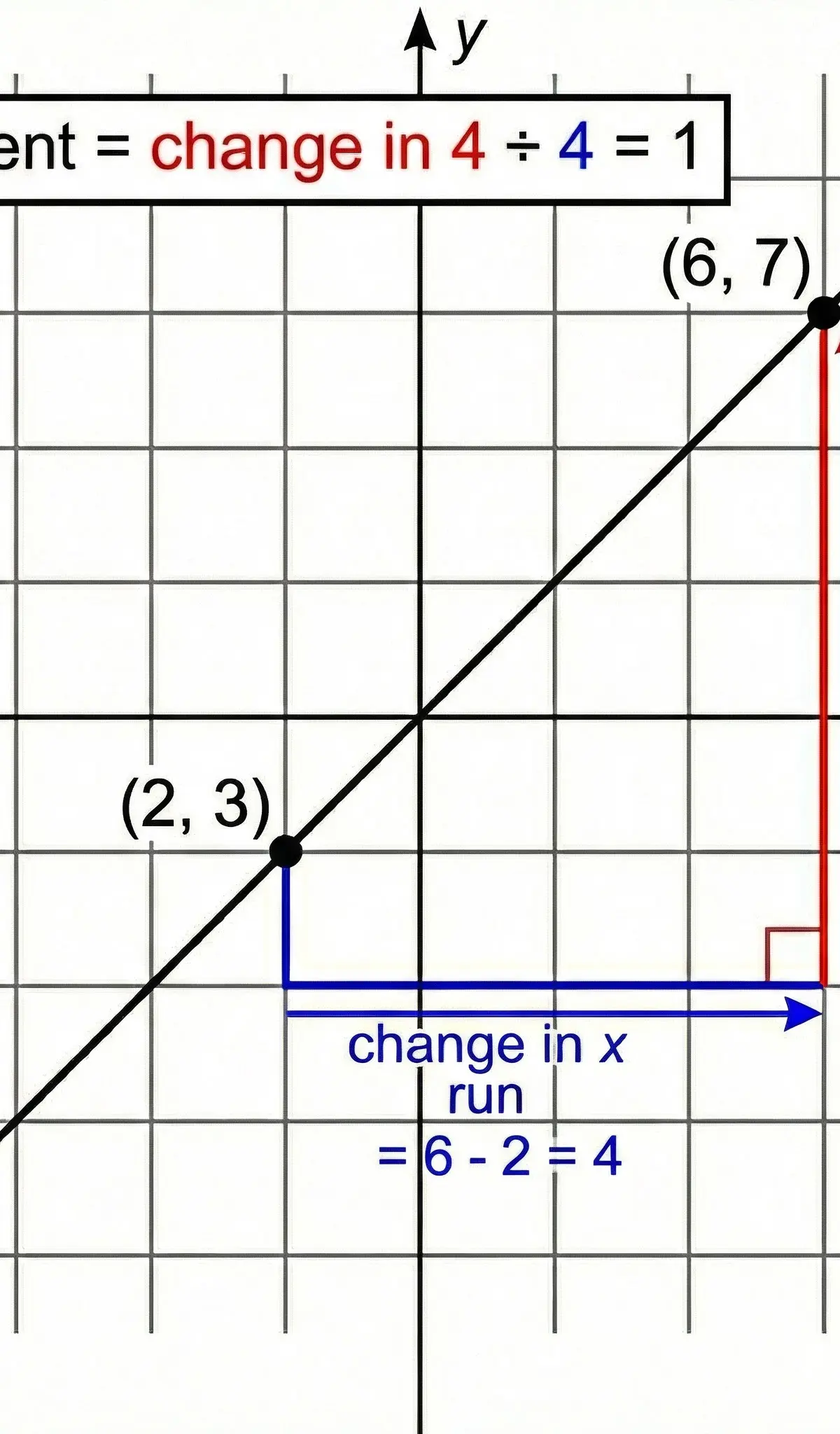
The gradient represents a rate of change. For a straight line, this rate is constant. For a curve, the rate of change is different at every point, which is why we use tangents.

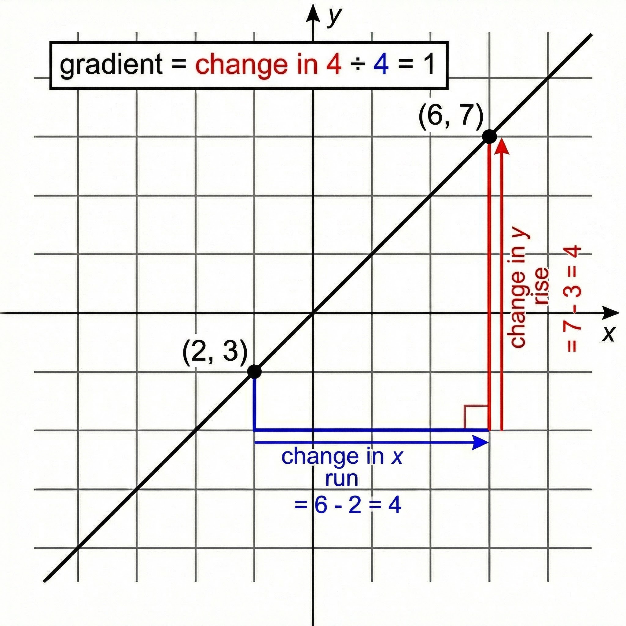
• Gradient of a Straight Line: Choose two points on the line that are far apart to maximise accuracy. Draw a right-angled triangle connecting them. The gradient is the vertical change (rise) divided by the horizontal change (run). Examiners award a method mark (M1) for a correctly drawn triangle on the graph.

• Gradient of a Curve (Higher Tier): To find the gradient at a specific point on a curve, you must draw a tangent. A tangent is a straight line that just touches the curve at that single point without crossing it. Once you have drawn the tangent accurately with a ruler, you calculate its gradient just as you would for any straight line. An M1 mark is awarded for a correctly drawn tangent at the specified x-value.

Mathematical/Scientific Relationships

• Linear Equation: y = mx + c (Must memorise)
• Quadratic Equation (General Form): y = ax² + bx + c (Given on formula sheet)
• Gradient Formula: m = (y₂ - y₁) / (x₂ - x₁) (Must memorise)
• Equation of a Vertical Line: x = c (where c is a constant) (Must memorise)
• Equation of a Horizontal Line: y = c (where c is a constant) (Must memorise)

Practical Applications

Graphs are not just abstract drawings; they model the real world. Examiners love to test your ability to apply your knowledge.

• Distance-Time Graphs: The gradient of the line represents the speed of an object. A horizontal line means the object is stationary. A straight diagonal line means constant speed. A curved line indicates acceleration or deceleration.
• Velocity-Time Graphs (Higher Tier): The gradient represents acceleration. The area under the graph represents the distance travelled. This is a crucial synoptic link to kinematics.
• Conversion Graphs: Used to convert between units, such as miles and kilometres, or pounds and euros. These are typically linear graphs where you read values from one axis to another.
• Financial Graphs: Used to model costs, revenues, and profits. For example, a mobile phone tariff might be represented by a fixed monthly charge (the y-intercept) plus a cost per gigabyte of data (the gradient).