Graphs — AQA GCSE Mathematics
Verified courseTeaching note checked against the official specification.
Graphs in AQA GCSE Mathematics covers plotting and interpreting linear, quadratic, cubic, reciprocal and exponential functions, as well as solving equations graphically and identifying key features such as roots, intercepts, turning points and asymptotes. Mastery requires accurate plotting, recognising shape families and using graphs to solve simultaneous equations and inequalities.
Graphs explained
Graphs covers 16 specification points, including work with coordinates in all four quadrants and Plot graphs of equations that correspond to….
Read the full explanation
Open a point below for its explanation and revision guidance.
work with coordinates in all four quadrants
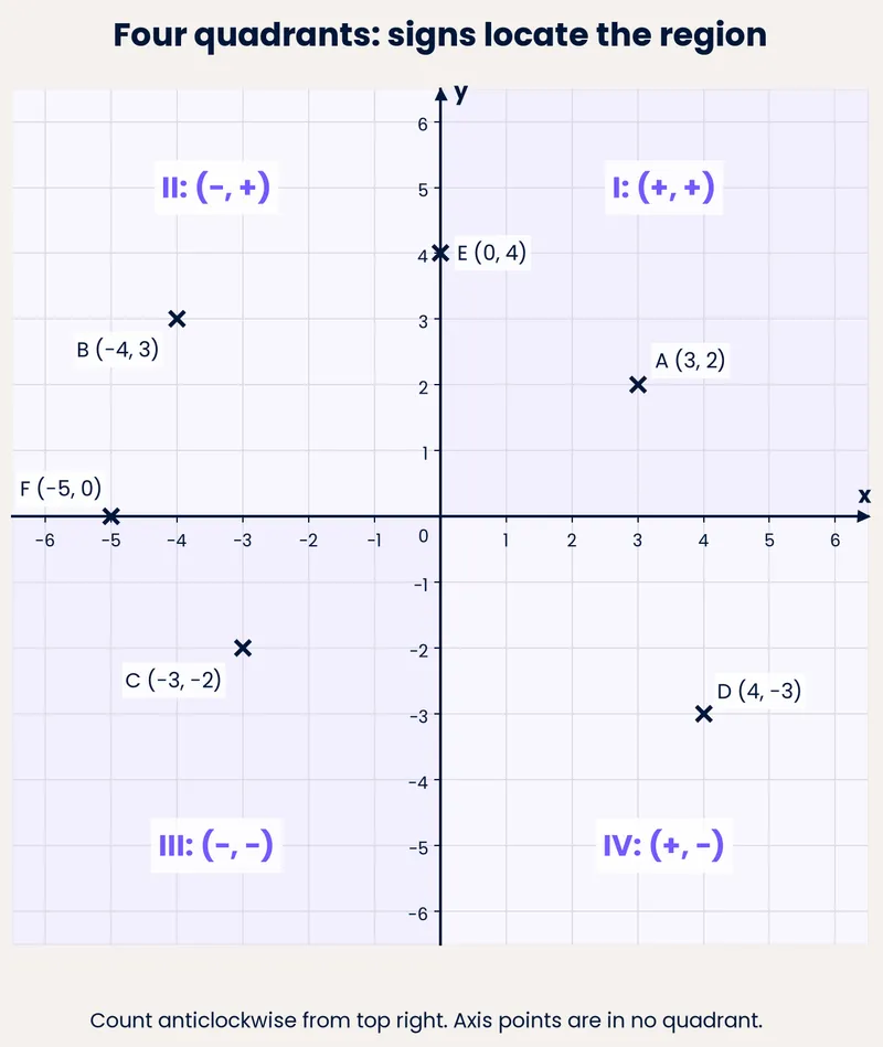
Coordinates locate a point using an ordered pair (x, y). The x-coordinate gives horizontal position from the origin: positive values lie to the right, negative values to the left. The y-coordinate gives vertical position: positive values lie above the origin, negative values below. The axes divide the plane into four quadrants. In the first quadrant both coordinates are positive; in the second x is negative and y is positive; in the third both are negative; in the fourth x is positive and y is negative. To plot (3, −2), move 3 units right from the origin, then 2 units down. To read a point, trace vertically to the x-axis for the first value and horizontally to the y-axis for the second. Reversing the order changes the point, so (3, −2) and (−2, 3) are different. Points on an axis have one coordinate equal to zero.
plot graphs of equations that correspond to straight-line graphs in the coordinate plane
An equation such as y = 2x + 1 pairs each x-value with exactly one y-value, producing a straight-line graph. To plot it, choose several x-values, substitute each into the equation to find the matching y-value, and record the results as coordinate pairs. For y = 2x + 1, x = 0 gives y = 1, so (0, 1) lies on the line; x = 2 gives y = 5, so (2, 5) lies on it. Plot the points on axes with a suitable scale, then draw a straight line through them with a ruler. A minimum of three points is a sensible check because a misplotted point will not lie on the straight line through the others. Equations of the form x = a produce vertical lines and y = b produce horizontal lines.
use the formy = mx + c to identify parallel lines find the equation of the line through two given points, or through one point with a given gradient
In the form y = mx + c, m is the gradient and c is the y-intercept. Parallel lines have equal gradients, so if two equations have the same m but different c, they are parallel. To find the equation of a line through two given points, first calculate the gradient using m = (y₂ − y₁)/(x₂ − x₁), then substitute one point into y = mx + c to find c. For example, through (1, 5) and (3, 11), m = (11 − 5)/(3 − 1) = 3, so 5 = 3(1) + c gives c = 2 and y = 3x + 2. Through one point with a given gradient, substitute the point and gradient directly to find c. Always check by substituting the other point.
use the form y = mx + c to identify perpendicular lines (Higher tier only)
For Higher tier, two straight lines are perpendicular if the product of their gradients is −1. In the form y = mx + c, if one line has gradient m, a perpendicular line has gradient −1/m (the negative reciprocal). For example, a line with gradient 2 is perpendicular to a line with gradient −1/2 because 2 × (−1/2) = −1. To identify perpendicular lines from equations, rearrange each into y = mx + c, read off the gradients, and check whether their product is −1. A horizontal line (gradient 0) is perpendicular to a vertical line, but vertical lines cannot be written in the form y = mx + c.
identify and interpret gradients and intercepts of linear functions graphically and algebraically
A linear function has the form y = mx + c. The gradient m measures steepness: it is the change in y divided by the change in x between two points, so m = (y₂ − y₁)/(x₂ − x₁). Intercepts are where the line crosses the axes. The y-intercept c is the y-value when x = 0. The x-intercept is the x-value when y = 0. Graphically, read intercepts where the line meets the axes and find the gradient by dividing vertical change by horizontal change between two points. Algebraically, rearrange into y = mx + c to identify m and c directly, and set y = 0 to find the x-intercept. For example, 3y = 6x + 9 becomes y = 2x + 3; the gradient is 2, the y-intercept is 3, and setting y = 0 gives x = -1.5.
identify and interpret roots, intercepts and turning points of quadratic functions graphically deduce roots algebraically
A quadratic function has the form y = ax² + bx + c and its graph is a parabola. The roots are the x-values where y = 0, so they are the x-intercepts of the curve. The y-intercept is the value of y when x = 0, which is c. The turning point is the vertex where the curve changes direction; it is a minimum when a is positive and a maximum when a is negative. Graphically, read roots where the curve crosses the x-axis, read the y-intercept where it crosses the y-axis, and read the turning point at the peak or trough. Algebraically, deduce roots by solving ax² + bx + c = 0, for example by factorising x² − 5x + 6 = 0 as (x − 2)(x − 3) = 0, giving roots x = 2 and x = 3.
deduce turning points by completing the square (Higher tier only)
Completing the square rewrites a quadratic from expanded form into vertex form, which exposes the turning point directly. For y = x² + bx + c, write y = (x + b/2)² + c − (b/2)². The squared bracket is never negative, so its least value is zero when x = −b/2; the y-value there is the constant term c − (b/2)². Hence the turning point is (−b/2, c − (b/2)²). For example, y = x² − 6x + 5 becomes y = (x − 3)² − 4, so the minimum is (3, −4). If the coefficient of x² is not 1, first factor it out of the x-terms, complete the square inside, then multiply back. A negative leading coefficient makes the bracket's contribution greatest at zero, giving a maximum. Deduction means reading the coordinates from the completed-square form, not plotting points.
recognise, sketch and interpret graphs of linear functions and quadratic functions
Linear functions have the form y = mx + c and graph as straight lines: m is the gradient and c is the y-intercept. Quadratic functions have the form y = ax² + bx + c and graph as parabolas; a > 0 opens upwards, a < 0 opens downwards, and the y-intercept is c. Recognising means matching an equation to its graph shape and key features. Sketching means drawing a clear curve or line with labelled intercepts, turning point and axis of symmetry where relevant, without needing exact plotting. Interpreting means reading information from a given graph, such as gradient, intercepts, roots and the turning point. For example, y = 2x − 3 is a line crossing the y-axis at −3 with gradient 2, while y = x² − 4 is a parabola crossing the x-axis at x = −2 and x = 2 with a minimum at (0, −4).
including simple cubic functions and the reciprocal function y = 1/x with x ≠ 0
Recognise, sketch and interpret graphs of simple cubic functions and the reciprocal function y = 1/x (where x ≠ 0). A simple cubic, y = ax³ + bx² + cx + d (a ≠ 0), has either two or no turning points. For example, y = x³ passes through the origin, rising steeply for positive x and falling steeply for negative x, with a stationary point of inflection at the origin, not a turning point. The reciprocal graph y = 1/x has two separate branches. As x approaches zero, y becomes very large, making the y-axis a vertical asymptote. As x becomes very large or small, y approaches zero, making the x-axis a horizontal asymptote. The domain excludes x = 0. You must be able to match these equations to their corresponding graphs.
including exponential functions y = kˣ for positive values of k, and the trigonometric functions (with arguments in degrees) y = sin x, y = cos x and y = tan x for angles of any size (Higher tier only)
This Higher tier point covers exponential graphs y = kˣ for positive k, and trigonometric graphs y = sin x, y = cos x and y = tan x in degrees. For y = kˣ with k > 1, the graph rises, passes through (0, 1) since k⁰ = 1, and has the x-axis as a horizontal asymptote. For 0 < k < 1, the graph falls but still passes through (0, 1). The trigonometric graphs are periodic: y = sin x and y = cos x have a period of 360° and range from −1 to 1. The graph of y = tan x has a period of 180° and is undefined at 90°, 270°, etc., where it has vertical asymptotes. You must recognise these shapes, state key features, and use them to solve simple trigonometric equations for angles of any size, including negative angles.
sketch translations and reflections of a given function (Higher tier only)
This Higher tier skill asks you to sketch, not plot point by point, the graph of a function after a translation or a reflection. Start from the given function y = f(x). A translation shifts the whole curve without turning it over: y = f(x) + a moves it a units up (a > 0) or down (a < 0), while y = f(x + a) moves it a units left when a > 0 and right when a < 0. A reflection flips the curve: y = −f(x) reflects it in the x-axis, and y = f(−x) reflects it in the y-axis. For example, if f(x) = x², then y = f(x) + 3 is the same parabola moved 3 units up, and y = f(−x) is unchanged because x² is even. You should mark key features such as intercepts, turning points and asymptotes, and label the new position clearly.
plot and interpret graphs, and graphs of non-standard functions in real contexts, to find approximate solutions to problems such as simple kinematic problems involving distance, speed and acceleration
This skill covers plotting graphs from data or equations, reading information from them, and using them to solve real problems. You may meet non-standard functions such as piecewise linear graphs, step graphs or curves that are not simple straight lines. In a kinematic context, a distance–time graph has gradient equal to speed, and a speed–time graph has gradient equal to acceleration and area under the graph equal to distance travelled. To find an approximate solution, plot or read the graph, identify the relevant point or interval, and estimate the value required. For example, from a speed–time graph you can estimate acceleration by drawing a tangent at a point, or estimate distance by counting squares under the curve. Always state the units and comment on whether the answer is reasonable in the context.
including reciprocal graphs
A reciprocal graph comes from an equation y = k/x, where k is a non-zero constant. Because division by zero is undefined, x cannot be zero, so the graph splits into two separate branches. For positive k, branches lie in the first and third quadrants; for negative k, they lie in the second and fourth. Each branch is a smooth curve that approaches, but never touches, the x-axis and y-axis, which act as asymptotes. As x increases, y approaches zero; as x approaches zero, the magnitude of y increases. The graph has no intercepts. To sketch it, plot points such as (1, k), (2, k/2), (0.5, 2k) and their negatives, then join them with smooth curves that flatten towards the axes without crossing them.
including exponential graphs (Higher tier only)
An exponential graph comes from an equation of the form y = aˣ, where a is a positive constant not equal to 1. For a > 1, the graph rises steeply as x increases and approaches the x-axis as x decreases, so the x-axis (y = 0) is a horizontal asymptote. For 0 < a < 1, the graph falls steeply as x increases and approaches the x-axis as x increases. The graph always passes through (0, 1) because a⁰ = 1 for any non-zero a. It has no x-intercept and never touches the x-axis. To sketch it, plot points such as (−1, 1/a), (0, 1), (1, a) and (2, a²), then join them with a smooth curve that flattens towards the x-axis on one side. This topic is for Higher tier only.
calculate or estimate gradients of graphs and areas under graphs (including quadratic and other non- linear graphs), and interpret results in cases such as distance-time graphs, velocity-time graphs and graphs in financial contexts (Higher tier only)
This Higher tier skill has two halves. To calculate a gradient, pick two points on the graph, form the right-angled triangle between them and divide the change in y by the change in x; for a curve this gives the gradient of the chord, and estimating the gradient at one point means drawing a tangent there and reading its slope. To estimate an area under a graph, split the region into strips, often trapezia, and add their areas; more, narrower strips improve the estimate. Interpretation matters: on a distance-time graph the gradient is speed, on a velocity-time graph the gradient is acceleration and the area under it is distance travelled, and in financial contexts a gradient can be a rate of change such as cost per unit while an area can represent total accumulated value.
recognise and use the equation of a circle with centre at the origin find the equation of a tangent to a circle at a given point (Higher tier only)
A circle with centre at the origin and radius r has equation x² + y² = r², so a point lies on the circle exactly when its coordinates satisfy that equation. To recognise the equation, compare the constant term with the square of the radius; for example x² + y² = 25 is a circle of radius 5 centred at the origin. To find the equation of a tangent at a given point, first find the gradient of the radius joining the origin to that point, then use the fact that the tangent is perpendicular to the radius, so its gradient is the negative reciprocal. Substitute the point's coordinates into y = mx + c, or use the point-gradient form, to obtain the tangent's equation.
Watch and listen
Listen: Graphs audio lesson
Read the full guideVisual Resources
1 diagram and illustration
Interactive Diagrams
1 interactive diagram to visualise key concepts
Conceptual Flow Outline
A reliable plotting routine: read, scale, locate x, locate y, mark, check.
Your focus
- State the quadrant of a point from the signs of its coordinates.
- Plot an ordered pair accurately in any of the four quadrants.
- Read the coordinates of a marked point and write them as an ordered pair.
Show all 48 objectives
- Complete a table of values for a linear equation by substitution.
- Plot the resulting coordinate pairs and draw the straight-line graph accurately.
- Identify and sketch vertical and horizontal lines from equations of the form x = a and y = b.
- Identify parallel lines from their equations in the form y = mx + c.
- Find the equation of a straight line passing through two given points.
- Find the equation of a straight line given one point and its gradient.
- Identify perpendicular lines from their equations in the form y = mx + c.
- Calculate the gradient of a line perpendicular to a given line.
- Use the condition m₁ × m₂ = −1 to test whether two lines are perpendicular.
- Find the gradient of a straight line from its graph or from two points.
- State the x-intercept and y-intercept of a straight line from its graph or equation.
- Rearrange a linear equation into the form y = mx + c and use it to identify the gradient and intercepts.
- Identify roots, intercepts and turning points of a quadratic function from its graph.
- Deduce the roots of a quadratic equation algebraically, for example by factorising.
- Interpret the turning point as a maximum or minimum and relate it to the shape of the parabola.
- Complete the square for a quadratic expression, including cases where the leading coefficient is not 1.
- Deduce the coordinates of the turning point from the completed-square form.
- Determine whether the turning point is a minimum or a maximum from the sign of the leading coefficient.
- Recognise linear and quadratic functions from their equations and graphs.
- Sketch linear and quadratic graphs showing key features such as intercepts, gradient and turning point.
- Interpret information from linear and quadratic graphs, including roots, intercepts and turning points.
- Sketch the graph of a simple cubic function and identify its key features.
- Sketch the graph of y = 1/x, stating that x ≠ 0 and describing its asymptotes.
- Match equations of cubic and reciprocal functions to their correct graphs.
- Sketch and interpret exponential graphs y = kˣ for positive k, identifying the asymptote and y-intercept.
- Sketch and interpret the graphs of y = sin x, y = cos x and y = tan x for angles in degrees, stating period and range.
- Solve simple trigonometric equations for angles of any size using graph or unit circle methods.
- Identify the transformation represented by y = f(x) + a, y = f(x + a), y = −f(x) and y = f(−x).
- Sketch the graph of a translated or reflected function from a given original graph.
- Mark and label key features of the transformed graph accurately.
- Plot a graph from given data or an equation and use it to answer questions about a real context.
- Interpret the gradient and area under distance–time and speed–time graphs to find speed, acceleration and distance.
- Find and justify approximate solutions to problems involving non-standard graphs.
- Identify the equation and key features of a reciprocal graph.
- Sketch the graph of y = k/x for positive and negative values of k, showing two separate branches.
- Explain why the graph has asymptotes at x = 0 and y = 0 and no intercepts.
- Identify the equation and key features of an exponential graph.
- Sketch the graph of y = aˣ for a > 1 and for 0 < a < 1, showing the correct shape and asymptote.
- Explain why the graph passes through (0, 1) and never crosses the x-axis.
- Calculate the gradient of a straight-line graph and estimate the gradient of a curve at a point using a tangent.
- Estimate the area under a curve by summing the areas of strips such as trapezia.
- Interpret gradients and areas in distance-time, velocity-time and financial contexts with correct units.
- Recognise and use the equation x² + y² = r² for a circle centred at the origin.
- Determine the gradient of a tangent at a point on a circle using perpendicularity to the radius.
- Find the equation of the tangent to a circle at a given point.
Graphs flashcards
Card 1 of 11
Exponential graph
Which command word is this?
Draw points accurately on a grid and join them appropriately (straight line for linear, smooth curve for non-linear).
Graphs exam tips
Topic Overview
Graphs is a fundamental topic in AQA GCSE Mathematics that involves representing relationships between variables visually. You will learn to plot and interpret linear, quadratic, cubic, reciprocal and exponential graphs, and use them to solve equations and inequalities. This topic connects algebra and geometry, and is essential for understanding functions and modelling real-world situations.
Graphs appear across both Foundation and Higher tiers, with Higher tier including more complex functions such as exponential graphs and transformations. Mastery of graphs is crucial for solving simultaneous equations, finding roots, and interpreting rates of change. It also provides a foundation for A-level Mathematics topics like calculus and functions.
Key Concepts
- →Linear graphs have the form y = mx + c, where m is the gradient and c is the y-intercept; they are straight lines.
- →Quadratic graphs have the form y = ax^2 + bx + c and are U-shaped (parabolas); the turning point and roots are key features.
- →Cubic graphs have the form y = ax^3 + bx^2 + cx + d and have an S-shape with up to three roots.
- →Reciprocal graphs have the form y = a/x and have two branches with asymptotes at x = 0 and y = 0.
- →Exponential graphs have the form y = k^x and show rapid growth or decay, passing through (0, 1) when k > 0.
Marking Points
- Identifies the quadrant from the signs of both coordinates: (positive, positive) is the first quadrant, (negative, positive) the second, (negative, negative) the third and (positive, negative) the fourth.
- Plots a given ordered pair correctly by moving horizontally by the x-coordinate and vertically by the y-coordinate from the origin.
- Reads the coordinates of a marked point as an ordered pair, taking the x-value from the horizontal axis first and the y-value from the vertical axis second.
- Recognises that reversing the order of the coordinates generally gives a different point, for example (3, −2) is not the same as (−2, 3).
- Handles coordinates on the axes, where one coordinate is zero, and states the axis on which such a point lies.
- Constructs a table of values by substituting chosen x-values into the equation and calculating the corresponding y-values correctly.
- Writes each pair of values as an ordered coordinate pair with the x-value first and the y-value second.
- Plots the coordinate pairs accurately on a coordinate grid using a consistent scale on each axis.
- Draws a single straight line through the plotted points with a ruler, extending it beyond the outermost points where the grid allows.
- Uses a third or further point as a check that the plotted points are collinear and corrects any point that does not fit the straight line.
- Recognises special cases: an equation of the form x = a gives a vertical line and y = b gives a horizontal line.
- State that in y = mx + c, m represents the gradient and c represents the y-intercept.
- Identify parallel lines by recognising that they have equal gradients (the same value of m).
- Calculate the gradient between two points using m = (y₂ − y₁)/(x₂ − x₁).
- Find c by substituting the coordinates of a given point and the gradient into y = mx + c.
- Form the equation of a line through one point with a given gradient by substituting the point and gradient to find c.
- Check the final equation by substituting the second point or the given point.
- State that perpendicular lines have gradients whose product is −1.
- Find the negative reciprocal of a given gradient to obtain the perpendicular gradient.
- Rearrange a linear equation into the form y = mx + c to identify its gradient.
- Check whether two lines are perpendicular by multiplying their gradients and testing whether the result is −1.
- Recognise that a horizontal line (gradient 0) is perpendicular to a vertical line, which cannot be written as y = mx + c.
- Gradient is the change in y divided by the change in x between two points on the line.
- The y-intercept is the value of y when x = 0, where the line crosses the y-axis.
- The x-intercept is the value of x when y = 0, where the line crosses the x-axis.
- In y = mx + c, m is the gradient and c is the y-intercept.
- An equation must be rearranged into the form y = mx + c before m and c can be read off.
- Roots of a quadratic are the x-values where the graph crosses the x-axis, that is where y = 0.
- The y-intercept of y = ax² + bx + c is the constant term c, at x = 0.
- The turning point is the vertex where the curve changes from decreasing to increasing or vice versa.
- A positive coefficient of x² gives a minimum turning point; a negative coefficient gives a maximum turning point.
- Roots can be deduced algebraically by solving the quadratic equation, for example by factorising.
- Rewrite the quadratic in the form a(x + p)² + q by completing the square, halving the coefficient of x inside the bracket and subtracting the square of that half from the constant.
- Identify the turning point as (−p, q) when the completed-square form is a(x + p)² + q, since the squared term is zero at x = −p.
- State whether the turning point is a minimum or a maximum: minimum when a > 0, maximum when a < 0.
- Handle a leading coefficient other than 1 by factoring it from the x-terms before completing the square, then restoring it correctly.
- Interpret the completed-square constant as the y-coordinate of the turning point, not the y-intercept.
- Identify a linear function from its equation or graph and state its gradient and y-intercept.
- Recognise a quadratic function from its equation or graph and identify the direction of opening from the sign of the coefficient of x².
- Sketch a straight-line graph using the gradient and y-intercept, or by plotting two convenient points.
- Sketch a quadratic graph showing the correct shape, y-intercept, roots where they exist, and turning point.
- Interpret key features from a graph, including intercepts, gradient, roots and the coordinates of the turning point.
- Recognises that a simple cubic function has the form y = ax³ + bx² + cx + d with a ≠ 0 and can sketch a typical cubic shape with two or no turning points.
- Identifies the reciprocal function y = 1/x and states that x ≠ 0, so the graph has no y-intercept and is undefined at x = 0.
- Describes the two branches of y = 1/x in the correct quadrants: for x > 0, y > 0, and for x < 0, y < 0.
- States that the x-axis and y-axis are asymptotes of y = 1/x, and explains that the curve approaches but never touches them.
- Matches a given equation or graph to its correct family, distinguishing a cubic from a reciprocal graph by shape and key features.
- Recognises that y = kˣ for k > 0 and k ≠ 1 passes through (0, 1) and has the x-axis as a horizontal asymptote; when k = 1 it is the constant line y = 1.
- Describes the shape of y = kˣ: increasing for k > 1, decreasing for 0 < k < 1, and never touching the x-axis; handles k = 1 as y = 1.
- States that y = sin x and y = cos x have period 360° and range −1 ≤ y ≤ 1, and sketches their wave shapes.
- States that y = tan x has period 180°, is undefined at 90° + 180°n, and has vertical asymptotes at those values.
- Uses the graphs to find all solutions in a given interval for equations such as sin x = 0.5 or tan x = 1, including angles of any size.
- Recognise that y = f(x) + a translates the graph vertically by a units, with a > 0 moving it up and a < 0 moving it down.
- Recognise that y = f(x + a) translates the graph horizontally by −a units, so a > 0 moves it left and a < 0 moves it right.
- Recognise that y = −f(x) reflects the graph in the x-axis, changing the sign of every y-coordinate.
- Recognise that y = f(−x) reflects the graph in the y-axis, changing the sign of every x-coordinate.
- Sketch the transformed curve with the correct shape and position, marking key points such as intercepts, turning points or asymptotes where relevant.
- Plot points accurately from a table or equation and draw a suitable graph, choosing sensible scales and labelling axes with units.
- Interpret the shape and key features of a graph in context, including intercepts, gradients, turning points and areas.
- For distance–time graphs, use the gradient to find speed and interpret horizontal sections as stationary periods.
- For speed–time graphs, use the gradient to find acceleration and the area under the graph to find distance travelled.
- Find approximate solutions by reading from the graph, drawing tangents or counting squares, and give answers with appropriate units.
- Comment on the accuracy of an approximate solution and whether it is reasonable in the real context.
- Recognise that a reciprocal graph has equation y = k/x with k ≠ 0 and that x = 0 is excluded from the domain.
- Identify the two separate branches and state the quadrant pair: first and third for k > 0, second and fourth for k < 0.
- State that the x-axis and y-axis are asymptotes that the curve approaches but never meets.
- Explain that the graph has no intercepts with either axis and that y is undefined at x = 0.
- Sketch the correct shape by plotting points such as (1, k), (2, k/2), (0.5, 2k) and their negative counterparts, then joining with smooth curves.
- Recognise that an exponential graph has equation y = aˣ with a > 0 and a ≠ 1.
- State that the graph passes through (0, 1) because a⁰ = 1.
- Identify the x-axis (y = 0) as a horizontal asymptote that the curve approaches but never meets.
- Describe the shape: for a > 1 the graph increases steeply as x increases; for 0 < a < 1 it decreases steeply as x increases.
- Sketch the graph by plotting points such as (−1, 1/a), (0, 1), (1, a) and (2, a²) and joining them with a smooth curve.
- Calculates a gradient from two points by dividing the change in y by the change in x, keeping the sign consistent with the direction of the graph.
- Estimates the gradient of a curve at a point by drawing a tangent at that point and finding the tangent's gradient from two points on it.
- Estimates the area under a curve by splitting the region into strips, commonly trapezia, and summing their areas.
- Explains that using more, narrower strips brings the estimate closer to the true area.
- Interprets the gradient of a distance-time graph as speed and the gradient of a velocity-time graph as acceleration.
- Interprets the area under a velocity-time graph as distance travelled.
- Interprets gradients and areas in financial contexts, for example a gradient as a rate of change and an area as an accumulated total.
- Recognises that x² + y² = r² represents a circle with centre at the origin and radius r.
- Uses the equation to test whether a given point lies on, inside or outside the circle.
- Finds the gradient of the radius from the origin to the given point on the circle.
- Uses perpendicularity to obtain the tangent gradient as the negative reciprocal of the radius gradient.
- Forms the equation of the tangent through the given point, for example by substituting into y = mx + c or using the point-gradient form.
- Handles special cases such as a point on an axis, where the radius is vertical or horizontal and the tangent is the other orientation.
Examiner Tips
- 💡Label the axes x and y before plotting, and mark the origin clearly so that negative movements are measured from the correct starting point.
- 💡Check the sign of each coordinate against the quadrant you expect: if you plot a point in the wrong region, one sign is probably reversed.
- 💡When reading a point from a grid, trace to both axes separately and write the pair in brackets with the x-value first, then verify by counting back to the point.
- 💡Choose x-values that are spread out, including zero and at least one negative value, so the line is checked across the grid rather than in one small region.
- 💡Show the substitution for at least one point so that an arithmetic slip can be identified and corrected.
- 💡After drawing the line, test one unplotted point from your table against the ruler edge to confirm it lies on the line.
- 💡Write down the formula y = mx + c and label m and c before starting any calculation.
- 💡When finding the equation through two points, calculate the gradient first and show your substitution clearly.
- 💡After finding an equation, substitute one of the given points to verify that both sides are equal.
- 💡Rearrange equations into y = mx + c before comparing gradients.
- 💡Write down the product of the two gradients to show clearly whether it equals −1.
- 💡Remember that the negative reciprocal of a whole number m is −1/m, and of a fraction a/b is −b/a.
- 💡Always rearrange an equation into y = mx + c before stating the gradient or y-intercept.
- 💡To find the x-intercept algebraically, substitute y = 0 into the equation and solve for x.
- 💡When reading from a graph, choose two points that lie exactly on grid intersections to reduce error.
- 💡Sketch the parabola to see where it crosses the axes and where the turning point lies.
- 💡When factorising to find roots, set each factor equal to zero and solve for x.
- 💡Check whether the turning point is a maximum or minimum by looking at the sign of the x² coefficient.
- 💡Show the completed-square form explicitly before stating the coordinates, so the deduction is visible to the examiner.
- 💡Check the sign of the x-coordinate by substituting it back into the original quadratic and confirming the y-value.
- 💡If the coefficient of x² is not 1, factor it out first and keep track of it through every line to avoid arithmetic slips.
- 💡State 'minimum' or 'maximum' with the coordinates, because the question asks for the turning point and its nature may be required.
- 💡Label the y-intercept and any roots on your sketch to show the key features clearly.
- 💡Use the sign of the coefficient of x² to decide whether the parabola opens upwards or downwards before drawing it.
- 💡For a linear graph, plot at least two points or use the gradient and y-intercept to ensure the line is straight and correctly positioned.
- 💡When interpreting a graph, read coordinates from the axes carefully and state units if the context provides them.
- 💡When sketching y = 1/x, draw both branches and label the asymptotes clearly; examiners look for the correct quadrants and the approach to the axes.
- 💡For cubic graphs, mark any intercepts you can find and show the general shape; do not waste time plotting many points if the question only asks for a sketch.
- 💡Check whether the question restricts the domain, especially for y = 1/x where x ≠ 0; state this restriction if asked to give the domain.
- 💡When sketching trigonometric graphs, mark the key points such as maximum, minimum and intercepts, and label the period clearly.
- 💡For exponential graphs, always mark the y-intercept at (0, 1) and draw the horizontal asymptote along the x-axis.
- 💡When solving trigonometric equations, use the graph or the unit circle to find all solutions in the required interval, and remember to include negative angles if the interval extends below 0°.
- 💡Identify the type of transformation first: a change outside the function affects y-values, while a change inside the brackets affects x-values.
- 💡Use a few key points from the original graph, transform their coordinates, and check that the new curve passes through them.
- 💡For reflections, remember that the shape stays the same but is turned over; check the direction of opening or the sign of the gradient.
- 💡Always label axes with quantity and unit, and choose a scale that makes the graph easy to read.
- 💡For kinematic problems, write down which graph you have and what its gradient and area represent before calculating.
- 💡When estimating from a curve, show your method clearly, such as the tangent you drew or the squares you counted.
- 💡Give answers with units and check they are sensible for the context, for example a speed that is not negative unless the context allows it.
- 💡When asked to sketch y = k/x, mark at least one point on each branch, such as (1, k) and (−1, −k), to show the correct quadrants.
- 💡Label the asymptotes or state clearly that the axes are asymptotes, because this is a key feature that distinguishes reciprocal from other graphs.
- 💡Check the sign of k before drawing: a positive k gives branches in the first and third quadrants, while a negative k gives branches in the second and fourth.
- 💡Use a smooth curve for each branch and do not join them across the y-axis; examiners look for two separate branches.
- 💡Always mark the point (0, 1) on your sketch, as it is a fixed feature of every exponential graph of the form y = aˣ.
- 💡State the equation of the asymptote, usually y = 0, to show you understand the limiting behaviour.
- 💡Plot at least three points, including one negative x-value, to establish the correct curvature.
- 💡Show the two coordinate pairs you used for a gradient, then substitute into the change in y divided by the change in x, so the method is visible even if arithmetic slips.
- 💡For an area estimate, state the strip width and show at least one strip's area calculation before summing, and comment on whether your estimate is likely to be an overestimate or underestimate.
- 💡When a graph is set in context, name the quantity each axis represents and give the gradient or area with its correct unit, such as metres per second or pounds.
- 💡Write down the radius gradient and the tangent gradient as separate steps before forming the tangent equation, so the perpendicular relationship is clearly shown.
- 💡Check your tangent equation by substituting the given point's coordinates; both sides should agree.
- 💡For a point on an axis, sketch the circle and tangent first, since the tangent is then a simple horizontal or vertical line.
- 💡Always label your axes and use a suitable scale; marks are awarded for correctly labelled axes and accurate plotting.
- 💡When drawing curves, use a sharp pencil and draw a smooth curve through the points; do not use a ruler for curves.
- 💡For graphical solutions, clearly state the coordinates of intersection points and check your answer by substitution.
Common Mistakes
- Reading or writing the coordinates in the wrong order. The correction is to remember that the x-coordinate always comes first, so a point 3 right and 2 down is written (3, −2), not (−2, 3).
- Treating a negative coordinate as a distance to the right or upwards. The correction is that a negative x-coordinate moves left from the origin and a negative y-coordinate moves down.
- Mixing up the quadrants by counting them clockwise. The correction is to count anticlockwise from the top-right region, so the second quadrant is top-left and the third is bottom-left.
- Plotting a point on an axis as though it were inside a quadrant. The correction is that a zero coordinate places the point on the x-axis or the y-axis, not in a quadrant.
- Substituting the chosen value into the wrong part of the equation, for example treating 2x + 1 as 2(x + 1). The correction is to multiply the x-value by 2 first and then add 1.
- Joining the plotted points with separate line segments rather than one straight line. The correction is to draw a single straight line through all the points with a ruler.
- Plotting the coordinate pair in reverse order. The correction is to plot the x-value along the horizontal axis first and the y-value on the vertical axis second.
- Assuming every equation gives a slanted line. The correction is to recognise that x = a is vertical and y = b is horizontal.
- Thinking that parallel lines have the same y-intercept rather than the same gradient; correct by comparing the coefficient of x (m) in each equation.
- Subtracting coordinates in the wrong order when finding the gradient, such as (y₁ − y₂)/(x₂ − x₁); correct by keeping the same order for both numerator and denominator.
- Substituting the x-coordinate for y or the y-coordinate for x when finding c; correct by replacing x and y with the coordinates of the given point in the correct positions.
- Forgetting to divide by the change in x when calculating the gradient; correct by using the full formula m = (y₂ − y₁)/(x₂ − x₁).
- Thinking that perpendicular lines have the same gradient; correct by using the negative reciprocal relationship m₁ × m₂ = −1.
- Forgetting the negative sign when finding the perpendicular gradient; correct by changing the sign as well as flipping the fraction.
- Assuming that any two lines with different gradients are perpendicular; correct by checking that the product of the gradients is exactly −1.
- Trying to write a vertical line in the form y = mx + c; correct by recognising that vertical lines have equations of the form x = k and are perpendicular to horizontal lines.
- Reading the gradient as the change in x divided by the change in y; correct this by always dividing the vertical change by the horizontal change.
- Treating the coefficient of x as the intercept; correct this by rearranging to y = mx + c and identifying c as the constant term.
- Confusing the x-intercept and y-intercept; correct this by remembering the x-intercept occurs when y = 0 and the y-intercept when x = 0.
- Ignoring the sign of the gradient when the line falls from left to right; correct this by checking whether y decreases as x increases.
- Confusing roots with the y-intercept; correct this by remembering roots are x-values where y = 0 and the y-intercept is where x = 0.
- Reading the turning point as a root; correct this by identifying the vertex as the maximum or minimum point, not necessarily on the x-axis.
- Forgetting that a quadratic may have no real roots if the graph does not cross the x-axis; correct this by checking whether the curve meets the x-axis at all.
- Assuming the turning point always lies on the y-axis; correct this by locating the vertex from the symmetry of the curve or by completing the square.
- Reading the turning point as (p, q) from (x + p)² + q; the correct x-coordinate is −p because the bracket equals zero when x = −p.
- Forgetting to subtract (b/2)² when completing the square, which changes the constant and gives the wrong y-coordinate.
- Assuming every turning point is a minimum; a negative leading coefficient produces a maximum, and the sign of a must be checked.
- Treating the constant term q as the y-intercept; the y-intercept is found by substituting x = 0 into the original expression.
- Confusing the gradient and y-intercept in y = mx + c; the coefficient of x is the gradient and the constant is the y-intercept.
- Drawing a quadratic as a straight line or with the wrong curvature; a quadratic must be a smooth parabola, not a V-shape or a line.
- Assuming a parabola always crosses the x-axis; it may have no real roots, one repeated root or two roots.
- Reading the turning point as the y-intercept; the turning point is the maximum or minimum, while the y-intercept occurs at x = 0.
- Thinking that y = 1/x can take the value x = 0: the function is undefined there, so the graph never crosses the y-axis and has a vertical asymptote at x = 0.
- Drawing y = 1/x as a single continuous curve through the origin: the correct graph has two separate branches in opposite quadrants and does not pass through the origin.
- Assuming every cubic graph has exactly two turning points: a real cubic has either two or no local turning points (a stationary point of inflection, as in y = x³, is not a turning point).
- Thinking that y = kˣ can be zero or negative: for positive k, kˣ is always positive; for k ≠ 1 the graph approaches but never touches or crosses the x-axis, while k = 1 gives y = 1.
- Believing that y = tan x is defined at 90°: tan 90° is undefined, so the graph has a vertical asymptote there, not a point.
- Assuming y = sin x and y = cos x have period 180°: their period is 360°, while y = tan x has period 180°.
- Thinking that y = f(x + a) moves the graph right when a is positive; the correction is that it moves left, because the input x must be smaller to produce the same output.
- Confusing y = −f(x) with y = f(−x); the correction is that y = −f(x) reflects in the x-axis (vertical flip) while y = f(−x) reflects in the y-axis (horizontal flip).
- Plotting many individual points instead of sketching the transformed shape; the correction is to move or flip the whole curve and then mark the key features.
- Confusing distance–time and speed–time graphs; the correction is to check the vertical axis label: gradient is speed on a distance–time graph but acceleration on a speed–time graph.
- Reading the gradient as a difference in y-values only; the correction is to divide the change in y by the change in x.
- Forgetting that area under a speed–time graph represents distance; the correction is to calculate or estimate the area and attach the correct unit.
- Using a straight-line formula for a curved graph; the correction is to draw a tangent at the required point or estimate the area by counting squares.
- Joining the two branches with a single continuous curve: the branches are separate because x = 0 is undefined, so they must be drawn as two disconnected curves.
- Drawing the curve crossing an axis: a reciprocal graph never touches or crosses either axis, because k/x can never equal zero and x can never equal zero.
- Treating the graph as a straight line through the origin: y = k/x is a curve with asymptotes, not a linear graph, so it must bend towards the axes.
- Assuming the graph exists at x = 0: substituting x = 0 gives division by zero, so there is no point on the graph there.
- Drawing the graph crossing the x-axis: an exponential graph never touches or crosses the x-axis, because aˣ is always positive for any real x.
- Assuming the graph passes through the origin: at x = 0, y = a⁰ = 1, so the y-intercept is (0, 1), not (0, 0).
- Treating the graph as a straight line: exponential growth or decay is curved, becoming steeper or flatter, not linear.
- Confusing the direction of the curve for 0 < a < 1: when the base is between 0 and 1, the graph decreases as x increases, unlike the a > 1 case.
- Dividing the change in x by the change in y instead of the change in y by the change in x; the correction is to keep the gradient as the vertical change divided by the horizontal change.
- Reading a tangent as if it passed through the curve's turning point rather than touching the curve at the required point; the correction is to draw the tangent so it touches at that point and is locally parallel to the curve there.
- Treating the area under a velocity-time graph as a speed or a gradient; the correction is that the area under a velocity-time graph represents distance travelled.
- Assuming a straight-line answer for a curved graph; the correction is that a curve's gradient changes from point to point, so a tangent or chord is needed.
- Reading the constant term as the radius rather than the radius squared; the correction is that x² + y² = 25 has radius 5, since 5² = 25.
- Using the radius gradient itself as the tangent gradient; the correction is that the tangent is perpendicular to the radius, so its gradient is the negative reciprocal.
- Forgetting the negative sign when taking the negative reciprocal, for example turning a radius gradient of 2 into a tangent gradient of 2 rather than −1/2.
- Substituting the origin instead of the given point when finding the tangent's intercept; the correction is that the tangent passes through the given point on the circle.
- Students often think that a quadratic graph is a straight line or that it can be drawn with straight segments; it must be a smooth curve.
- Students may confuse the gradient and y-intercept when identifying the equation of a straight line; remember y = mx + c, where m is gradient and c is y-intercept.
- Students sometimes believe that reciprocal graphs cross the axes; they do not, as they have asymptotes at x = 0 and y = 0.
Revision Plan
- 1Week 1: Revise plotting linear graphs using tables of values and identifying gradient and y-intercept. Practice drawing straight lines from equations.
- 2Week 1: Move on to quadratic graphs; practice completing tables of values, plotting points, and drawing smooth curves. Identify roots and turning points.
- 3Week 2: Study cubic and reciprocal graphs; focus on their shapes and key features. Practice sketching them from equations.
- 4Week 2: Learn to solve simultaneous equations graphically and use graphs to solve quadratic equations. Attempt past paper questions.
- 5Week 2: Review exponential graphs and transformations of graphs if studying Higher tier. Complete a mixed topic test.
Exam Question Types
- 📋Plotting a graph from a table of values: Ensure you plot points accurately and join with a smooth curve for non-linear graphs.
- 📋Solving simultaneous equations graphically: Draw both lines and read off the intersection point; give both coordinates.
- 📋Using a graph to solve an equation: Find the x-intercepts for equations of the form f(x) = 0, or draw a new line for f(x) = k.
- 📋Identifying key features of a graph: State roots, intercepts, turning points, and asymptotes as required.
Command Word Expectations (AQA)
Draw points accurately on a grid and join them appropriately (straight line for linear, smooth curve for non-linear).
Draw a rough graph showing the correct shape and key features, without needing exact plotting.
Find the value(s) that satisfy the equation, often by reading from a graph or using algebraic methods.
How Students Lose Marks (Examiner Pitfalls)
Step-by-Step Worked Solutions
Question: Complete the table of values for y = x^2 - 2x - 3 for x = -2 to 3, then plot the graph and use it to solve x^2 - 2x - 3 = 0.
- 1.Step 1: Substitute each x value into y = x^2 - 2x - 3. For x = -2: y = 4 + 4 - 3 = 5; x = -1: y = 1 + 2 - 3 = 0; x = 0: y = -3; x = 1: y = 1 - 2 - 3 = -4; x = 2: y = 4 - 4 - 3 = -3; x = 3: y = 9 - 6 - 3 = 0.
- 2.Step 2: Plot the points (-2, 5), (-1, 0), (0, -3), (1, -4), (2, -3), (3, 0) on a grid and join with a smooth curve.
- 3.Step 3: The solutions to x^2 - 2x - 3 = 0 are the x-intercepts where y = 0. From the graph, the curve crosses the x-axis at x = -1 and x = 3.
Question: Solve the simultaneous equations y = 2x + 1 and y = -x + 4 graphically.
- 1.Step 1: Create a table of values for each equation. For y = 2x + 1: when x = 0, y = 1; when x = 2, y = 5. For y = -x + 4: when x = 0, y = 4; when x = 3, y = 1.
- 2.Step 2: Plot both straight lines on the same axes using the points from the tables.
- 3.Step 3: Identify the point where the two lines intersect. The lines cross at (1, 3). Check: 2(1) + 1 = 3 and -(1) + 4 = 3.